- Qingyun Wang
wangqingyun@pku.edu.cn - Jiaying Liu
liujiaying@pku.edu.cn - Wenhan Yang
yangwenhan@pku.edu.cn - Zongming Guo
guozongming@pku.edu.cn
Published on ICIP, September 2015
Overview
Image interpolation is a technique that rescales a low-resolution (LR) image to a high-resolution (HR) version.Conventional methods, such as Bilinear and Bicubic interpolations, apply a convolution to every pixel of the LR image. However, as these methods do not capture the fast varying property around edges and texture structures, aliasing, blurring and ringing artifacts occur in high frequency regions
To better model the essential property of edge regions, the explicit adaptive interpolation methods spring up.These methods, Like SAGA[1], utilize the structural information in an explicit way. They estimate the directions of edges and isophotes, and interpolate in these directions.However, when it comes to the images containing lots of complex structures, the isophotes estimated with these methods tend to be unpredictable, which increases the variation of the interpolation.
Instead of the explicit utilization of local structures, the implicit adaptive methods, embed these structures into the objective function and interpolate by optimizing it.A typical achievement is the autoregressive (AR) model. Li and Orchard [2] proposed a new edge-directed interpolation (NEDI). They estimate the model parameters according to the geometric duality and reconstruct the HR pixels with corresponding LR scale parameters. In [3], the soft-decision adaptive interpolation (SAI) adds a cross-direction constraint in the AR model and estimates HR pixels jointly rather than separately, which contributes to the better performance upon NEDI. However, these algorithms are generally based on the stationarity assumption in images, which does not hold on account of the diversification of natural images. Aiming to model the non-stationarity of image signals, our previous work IPAR [4] and an adaptive general scale interpolation [5] proposed similarity probability models. Due to getting rid of the global stationarity assumption, weighted AR methods raise the precision of interpolation and better characterize the piecewise stationarity of images.
Autoregressive (AR) Model
The autoregressive model is an effective tool for the image modeling. It models and predicts missing pixels based on the locality and stationarity. For instance, in the form of AR model, pixels in images are estimated by their adjacent neighbors with certain weights as follow:
![]()
where ![]() is the model parameter.
is the model parameter. ![]() is the adjacent neighbor of the pixel I(m,n). ε is the fitting error.
is the adjacent neighbor of the pixel I(m,n). ε is the fitting error.
To estimate precisely, two kinds of model parameters, those in cross directions and diagonal directions, are set up and estimated respectively in a rectangle local window.
Image Interpolation Based On Adaptive AR Model with Window Extension via Explicit Geometry
Our interpolation algorithm consists of four stages. First, we extend the interpolation window in the isophote direction. Second, we establish the similarity model. Third, we estimate the model parameters, and last, we obtain the center pixel of the interpolation window.

Fig.1. The flowchart of the proposed interpolation algorithm
3.1.Geometry-Aware Adaptive Window-Extension
Geometry information in the local region provides hints for the interpolation. A useful clue is the self-similarity along the isophote: patches located along the same isophote are similar with each other, and the information contained in adjacent similar patches may benefit the interpolation of target pixel. So the model estimates the isophote and then extends the interpolation window in the isophote direction. However, the exceptions of high curvature should be paid attention to. Due to the high curvature, any extension introduces the pixels whose AR parameters are not consistent with the central one. Thus, before the extension, we calculate the curvature of the center pixel and eliminate the extension in the high curvature situation. The curvature is calculated as:
![]()
If K is less than T, we choose a direction and extend the window. In our algorithm, the threshold T is adaptive to the angle θ between isophote and horizontal line as follow:
![]()
As for the extension details, there are 8 directions to be chosen as the extension direction. For convenience, we define the set of direction angels M as {0°, 27°, 45°, 63°, 90°, 117°, 135°, 153°}. And we use the θ mentioned above to estimate extension direction and, like the method in [1], make use of the definition of isophote to calculate θ. If the intensity function is treated as locally planar, intensities at arbitrary locations can be estimated based on the collected data and their first-order derivatives:
![]()
Specially,
![]()
Here the isophote is approximated locally with a line of constant intensity such that:
![]()
So,
![]()
And θ can be calculated as:
![]()
Finally, we use θ to find the most approximate angle in M as the extension direction.
3.2.Patch-Geodesic Distance Based Similarity
Since the global stationarity is not valid in some regions, the piecewise stationarity in natural images is regarded as the basis of the AR parameter estimation. To better characterize the piecewise stationarity in the local region, a novel similarity metric is proposed, combining the spatial distance with the pixel intensity distance and modulating them into the AR model. Like the method in [6], we let c denote the center pixel and x denote one pixel in the interpolation window. The patch-geodesic distance D(x,c) is defined as the minimum value of the patch differences along all paths:

where ![]() stands for the set of all paths connecting x and c. N ={1,2,…,8} contains all the neighboring indices of 8-neighbors.
stands for the set of all paths connecting x and c. N ={1,2,…,8} contains all the neighboring indices of 8-neighbors. ![]() is the j-th neighbor of the i-th pixel in P and the
is the j-th neighbor of the i-th pixel in P and the ![]() stands for the intensity of
stands for the intensity of ![]() . After obtaining patch-geodesic distance, we convert it to the similarity metric:
. After obtaining patch-geodesic distance, we convert it to the similarity metric:
![]()
where β is a user-defined parameter controlling the importance of distance weight.
3.3.Similarity Modulated Block Estimation
Acording to the AR model mentioned above, we minimize the fitting error of the pixels in the window W by solving the linear least squares problem:

Let x and y be the vectors consisting of the LR and HR pixels in W respectively. Let C and D be the vectors consisting of the covariance between pixels. Let S be the diagonal matrix composed of the similarity probability. We can deduce the objective function to a vector form:
![]()
Then a close-formed resolution can be obtained:
![]()
3.4.Weighted Ridge Regression with Parameter Estimation
We can estimate model parameters by solving the linear least squares problem:
And we can also deduce the objective function to a vector form:
![]()
However, in the presence of typical piecewise stationarity, the patterns of the model parameters are simple. Multicollinearity may exist between the model parameters. It results in the expansion of variance, which means the undesirable precision of the estimation.A method in [7] introduces weighted ridge regression (WRR) to reduce the influence of multicollinearity. The weighted ridge regression modulates weights into the regression to value the reliability of each sample, leading to more reliable estimations.
![]()
And it can be converted to a vector form:
![]()
Experimental Results
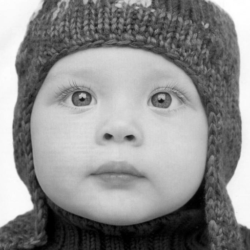
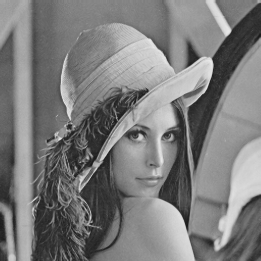
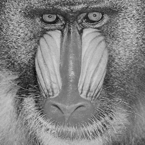
The proposed interpolation algorithm is implemented on MATLAB 7.6 platform and compared with conventional Bicubic interpolation method and three state-of-the-art interpolation methods: new edge-directed interpolation (NEDI) in [2], soft-decision adaptive interpolation (SAI) in [3] and similarity modulated block estimation for image interpolation(IPAR) in [4].We test the proposed algorithm on a large image set, including the Kodak database, many standard test images and some piecewise smooth images.
Table 1 tabulates the PSNR results of the five interpolation methods on several standard test images for 2X enlargement. To see the interpolated image of each method, please click the corresponding hyperlink of the PSNR number.The PSNR gains of the proposed method over the best method of other four methods(Bicubic, NEDI, SAI and IPAR) are also given in the parenthesis.
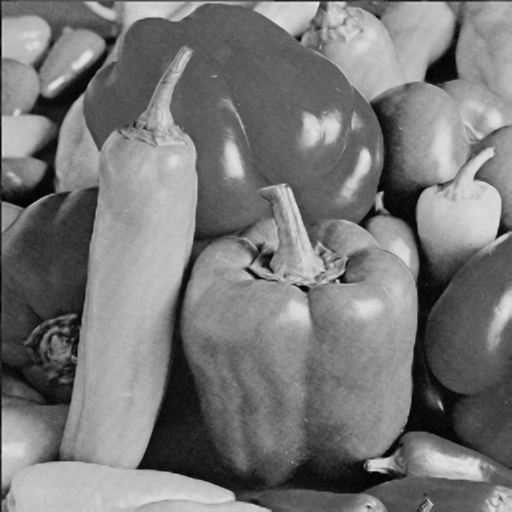
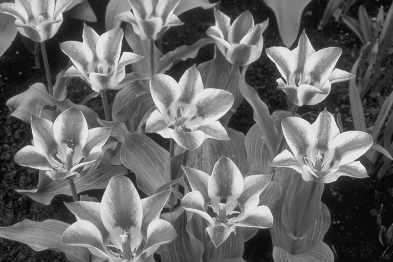
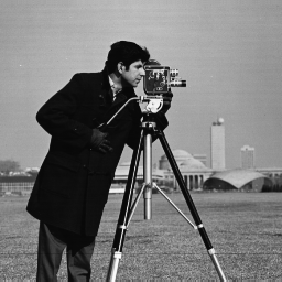
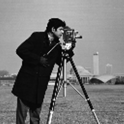
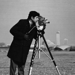
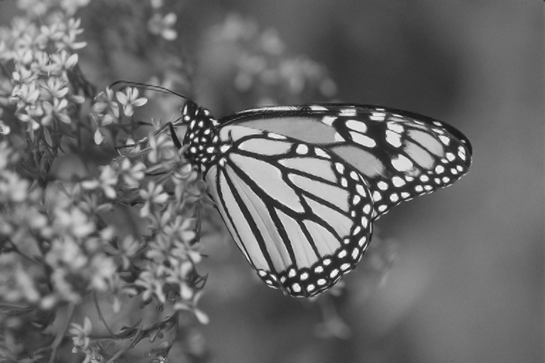
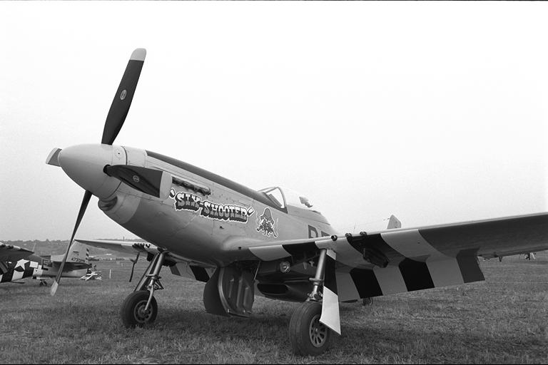
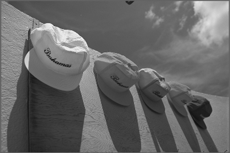
Table 1. PSNR(dB) results of five interpolation methods on standard test images.
| Images | Bicubic | NEDI[2] | SAI[3] | IPAR[4] | Proposed |
|---|---|---|---|---|---|
| child | 35.49 | 34.56 | 35.63 | 35.70 | 35.72 (0.02) |
| Lena | 34.01 | 33.72 | 34.76 | 34.79 | 34.80 (0.01) |
| Baboon | 22.47 | 22.55 | 22.70 | 22.69 | 22.71 (0.01) |
| Pepper | 32.06 | 29.32 | 31.84 | 32.69 | 32.69 (0.00) |
| Tulip | 33.82 | 33.76 | 35.71 | 35.85 | 35.81 (-0.04) |
| Cameraman | 25.51 | 25.44 | 25.99 | 26.06 | 26.13 (0.07) |
| Monarch | 31.93 | 31.80 | 33.08 | 33.34 | 33.31 (-0.03) |
| Airplane | 29.40 | 28.00 | 29.62 | 30.05 | 30.06 (0.01) |
| Caps | 31.25 | 31.19 | 31.64 | 31.67 | 31.68 (0.01) |
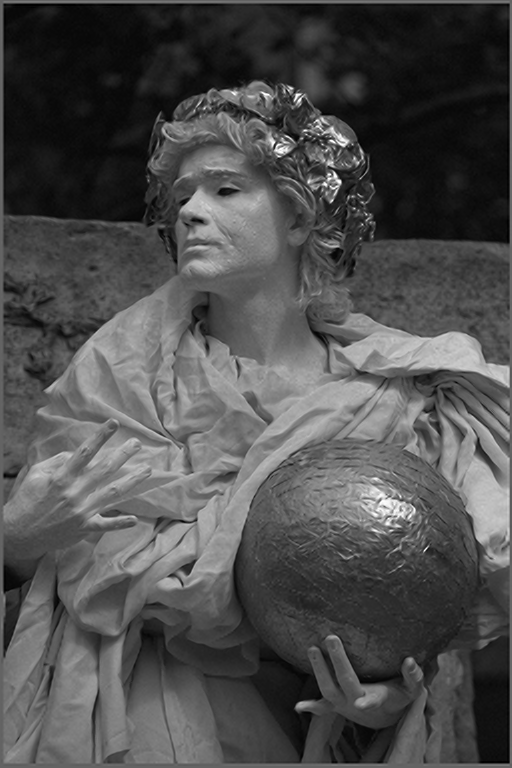
| Statue | 31.36 | 31.01 | 31.78 | 31.94 | 31.96 (0.02) |
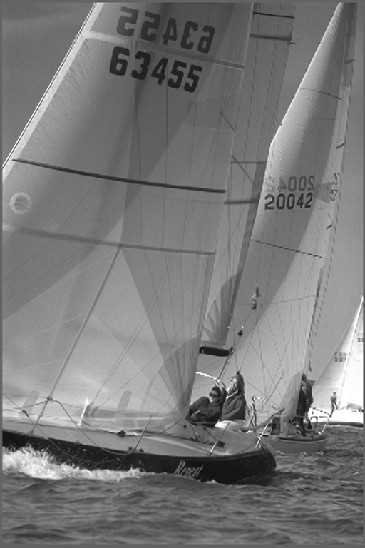
| Sailboat | 30.12 | 30.18 | 30.69 | 30.85 | 30.88 (0.03) |
| House | 22.20 | 21.74 | 22.28 | 22.33 | 22.39 (0.06) |
| Woman | 31.17 | 30.73 | 31.27 | 31.34 | 31.37 (0.03) |
| Bike | 25.41 | 25.25 | 26.28 | 26.31 | 26.31(0.00) |
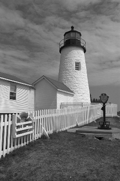
| lighthouse | 26.97 | 26.37 | 26.70 | 26.76 | 26.88(-0.09) |
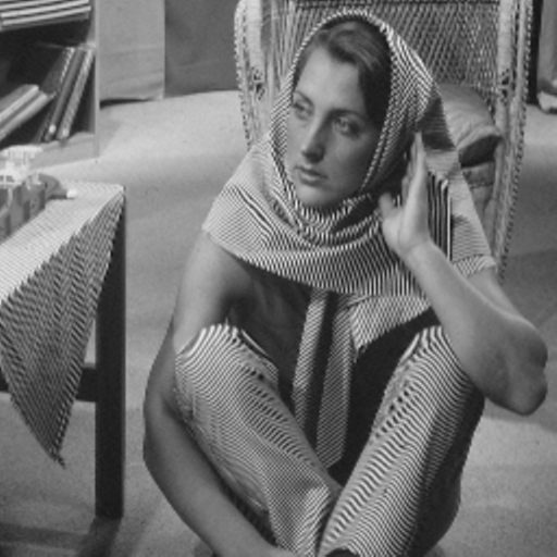
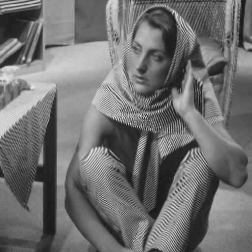
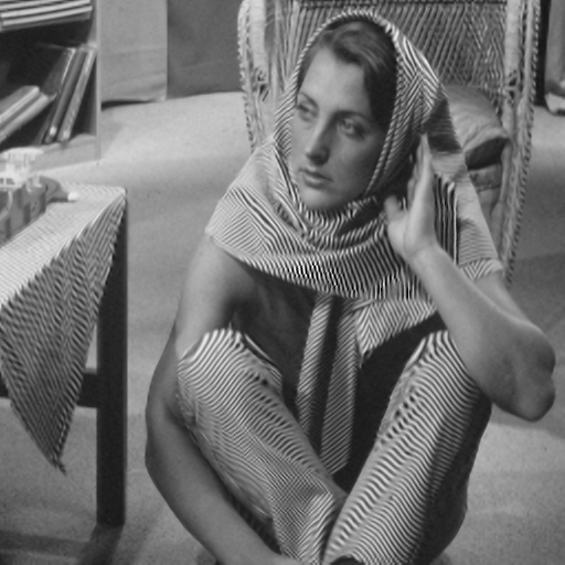
| barbara | 24.46 | 22.36 | 23.55 | 23.10 | 24.34 (-0.12) |
| Average | 29.23 | 28.62 | 29.60 | 29.72 | 29.82(0.10) |
Table 2 shows the PSNR results of the five interpolation methods on several piecewise smooth images for 2X enlargement. To see the interpolated image of each method, please click the corresponding hyperlink of the PSNR number.
Table 2. PSNR(dB) results of five interpolation methods on piecewise smooth images.
| Images | Bicubic | NEDI[2] | SAI[3] | IPAR[4] | Proposed |
|---|---|---|---|---|---|
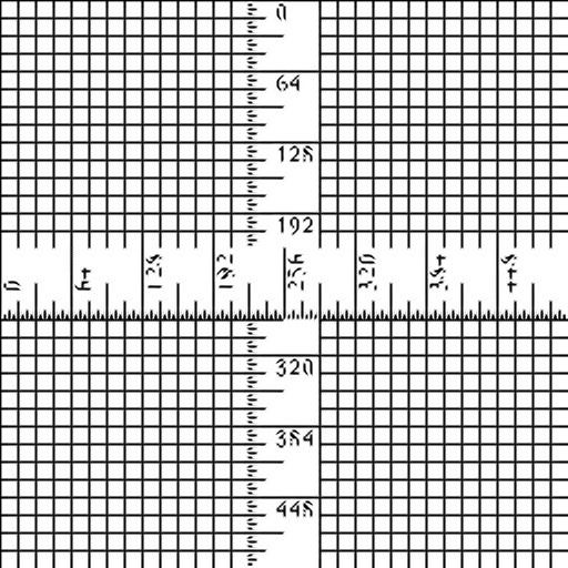
| Ruler | 11.98 | 11.49 | 11.37 | 11.81 | 12.43(0.45) |
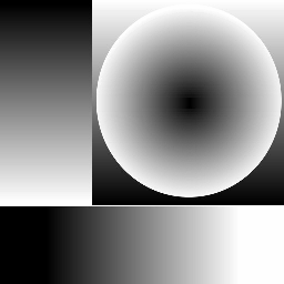
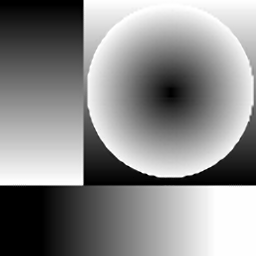
| Slope | 26.74 | 26.54 | 26.63 | 26.78 | 27.14(0.36) |
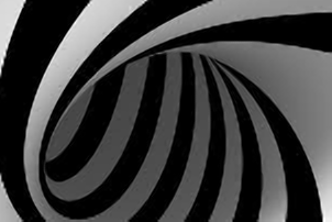
| rotateStripe | 29.75 | 29.25 | 30.79 | 33.15 | 33.24(0.09) |
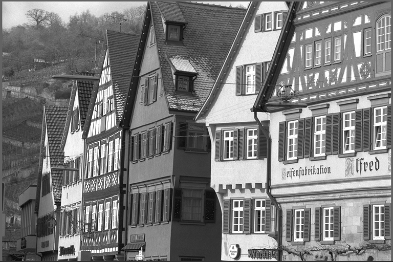
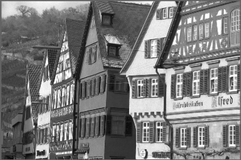
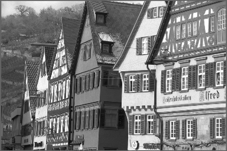
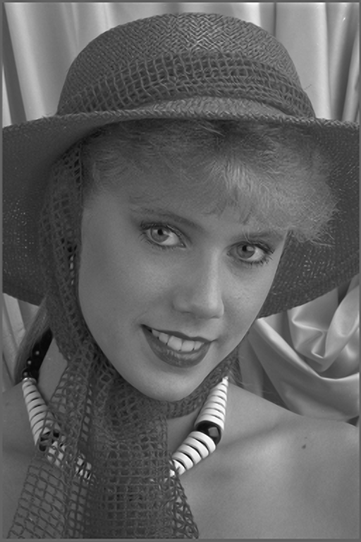
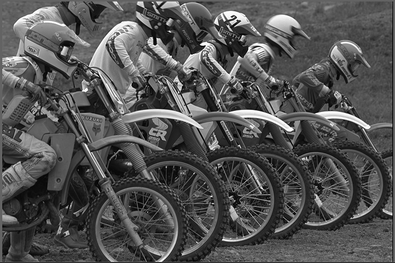
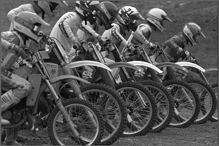
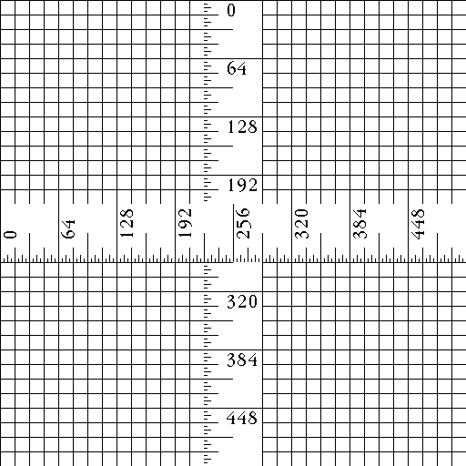
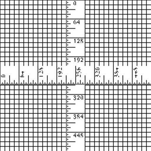
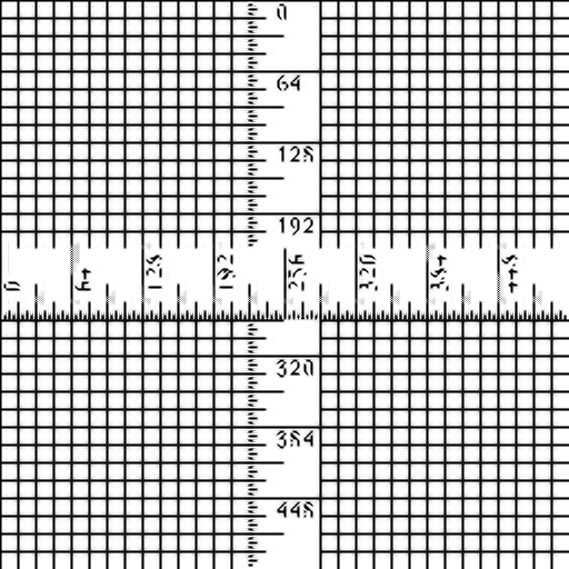
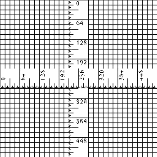
Fig 2 shows the visual comparisons of the five interpolation methods
 |
 |
 |
 |
 |
 |
Fig.2. Visual comparisons: Portions from various interpolated images using different methods. From top to bottom: Barbara, Ruler and Slope. From left to right: ground truth, Bicubic, NEDI, SAI, IPAR, proposed method.
References
[1] Christine M. Zwart and David H. Frakes, “Segment adap-tive gradient angle interpolation,” IEEE Transactions on Image Processing, vol. 22, no. 8, pp. 2960–9, 2013.
[2] Xin Li and Michael T. Orchard, “New edge-directed in-terpolation,” IEEE Transactions on Image Processing, vol. 10, no. 10, pp. 1521–7, 2001.
[3] Lei Zhang and Xiaolin Wu, “An edge-guided image inter-polation algorithm via directional filtering and data fusion,” IEEE Transactions on Image Processing, vol. 15, no. 8, pp. 2226–38, 2006.
[4] Jie Ren, Jiaying Liu, Wei Bai, Zongming Guo, “Similarity modulated block estimation for image interpolation”, IEEE International Conference on Image Processing (ICIP), Brus-sels, 2011.
[5] Mading Li, Jiaying Liu, Jie Ren, and Zongming Guo, “Adap-tive general scale interpolation based on similar pixels weighting,” IEEE International Symposium on Circuits and Systems (ISCAS) , Beijing, pp. 2143–2146, 2013.
[6] Tang Ketan, Oscar C. Au, Guo Yuanfang, Pang Jiahao, and Li Jiali, “Arbitrary factor image interpolation using geodesic distance weighted 2d autoregressive modeling,” IEEE inter-national Conference on Acoustics, Speech and Signal Pro-cessing (ICASSP), Vancouver, pp. 2217-2221, 2013
[7] Jian-Wu Xu, Shipeng Yu, Jinbo Bi, Lucian Vlad Lita, Radu Stefan Niculescu and R. Bharat Rao.” Automatic Medical Coding of Patient Records via Weighted Ridge Regression.” International Conference on Machine Learning and Appli-cations (ICMLA), pp.260-265, Ohio, Dec. 2007.