Submitted to IEEE Transaction on Image Processing (TIP)
- Wenhan Yang
yangwenhan@pku.edu.cn - Jiashi Feng
elefjia@nus.edu.sg - Jianchao Yang
jyang29@ifp.uiuc.edu - Fang Zhao
elezhf@nus.edu.sg - Jiaying Liu
liujiaying@pku.edu.cn - Zongming Guo
guozongming@pku.edu.cn - Shuicheng Yan
eleyans@nus.edu.sg

Fig.1. The framework of the proposed DEGREE network for image SR. The DEGREE network takes the raw LR image
as well as prior map (LR edge here) as its inputs and outputs the predicted HR feature maps and HR edge maps – which are
integrated to produce the HR image. The recurrent residual network (highlighted in orange color) recovers sub-bands of the
HR image features from the LR input iteratively and actively utilizes edge feature guidance in image SR for preserving sharp
details.
Abstract
In this work, we consider the image super-resolution (SR) problem. The main challenge of image SR is to recover high-frequency details of a low-resolution (LR) image that are important for human perception. To address this essentially ill-posed problem, we introduce a Deep Edge Guided REcurrent rEsidual (DEGREE) network to progressively recover the high-frequency details. Different from most of existing methods that aim at predicting high-resolution (HR) images directly, DEGREE investigates an alternative route to recover the difference between a pair of LR and HR images by recurrent residual learning. DEGREE further augments the SR process with edge-preserving capability, namely the LR image and its edge map can jointly infer the sharp edge details of the HR image during the recurrent recovery process. To speed up its training convergence rate, by-pass connections across multiple layers of DEGREE are constructed. In addition, we offer an understanding on DEGREE from the view-point of sub-band frequency decomposition on image signal and experimentally demonstrate how DEGREE can recover different frequency bands separately. Extensive experiments on three benchmark datasets clearly demonstrate the superiority of DEGREE over well-established baselines and DEGREE also provides new state-of-the-arts on these datasets. We also present addition experiments for JPEG artifacts reduction to demonstrate the good generality and flexibility of our proposed DEGREE network to handle other image processing tasks.
Contributions
1) We introduce a novel DEGREE network model to solve image SR problems. The DEGREE network integrates edge priors and performs image SR recurrently, and improves the quality of produced HR images in a progressive manner. Moreover, DEGREE is end-to-end trainable and thus effective in exploiting edge priors for both LR and HR images. With the recurrent residual learning and edge guidance, DEGREE outperforms well-established baselines significantly on three benchmark datasets and provides new state-of-the-arts.
2) The proposed DEGREE also introduces a new framework that is able to seamlessly integrate useful prior knowledge into a deep network to facilitate solving various image processing problems in a principled way. By letting certain middle layers in the DEGREE alike framework learn features reflecting the priors, our framework gets rid of hand-crafting new types of neurons for different image processing tasks based on domain knowledge, and thus is highly flexible to integrate useful priors into deep SR and other tasks.
3) To the best of our knowledge, we are the first to apply recurrent deep residual learning for SR, and we establish the relation between it and the classic sub-band recovery. Our extensive experimental results demonstrate that the recurrent residual structure is more effective in image SR than the standard feed forward architecture used in the modern CNN models. This is promising for providing new ideas for the community on how to design an effective network for SR or other tasks based on well-built traditional methods.
DEGREE Network
Recurrent Residual Network with Edge Guidence
We propose an end-to-end trainable deep edge guided recurrent residual network (DEGREE) for image
SR. The network is constructed based on the following two intuitions. First, as we have demonstrated, a
recurrent residual network is capable of learning sub-band decomposition and reconstruction for image
SR. Second, modeling edges extracted from the LR image would benefit recovery of details in the
HR image. An overview on the architecture of the proposed DEGREE network is given in Figure 2.
As shown in the figure, DEGREE contains following components. a) LR Edge Extraction. An edge
map of the input LR image is extracted by applying a hand-crafted edge detector and is fed into the
network together with the raw LR image, as shown in Figure 2(a). b) Recurrent Residual Network.
The mapping function from LR images to HR images is modeled by the recurrent residual network as
introduced in Section III-B, Instead of predicting the HR image directly, DEGREE recovers the residual
image at different frequency sub-bands progressively and combine them into the HR image, as shown in
Figure 2(b). c) HR Edge Prediction. DEGREE produces convolutional feature maps in the penultimate
layer, part of which (f edge ) are used to reconstruct the edge maps of the HR images and provide extra
knowledge for reconstructing the HR images, as shown in Figure 2(c). d) Sub-Bands Combination
For Residue. Since the LR image contains necessary low-frequency details, DEGREE only focuses on
recovering the high-frequency component, especially several high-frequency sub-bands of the HR image,
which are the differences or residue between the HR image and the input LR image. Combining the
estimated residue with sub-band signals and the LR image gives an HR image, as shown in Figure 2(d). e) Training Loss. We consider the reconstruction loss of both the HR image and HR edges simultaneously
for training DEGREE as shown in Figure 2(e).
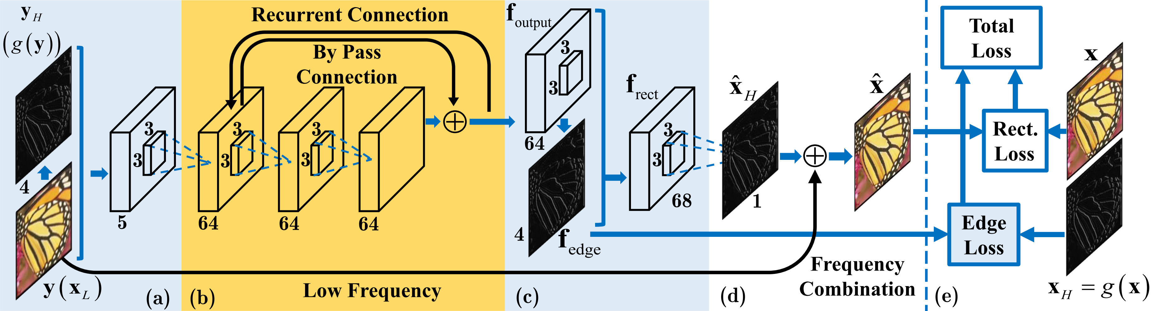
Fig.2. Representations of steerable pyramid transform with one scale and two orientations. From left to right: high-pass image, two directional sub-bands (vertical and horizontal, respectively ), and low-pass residue.
Connection to Sub-Band Recovery
Learning Sub-Band Decomposition by Recurrent Residual Net
The sub-band paradigm mentioned above learns to recover HR images through minimizing a hierarchical loss generated by applying hand-crafted frequency domain filters, as shown in Figure 3(a). However, this paradigm suffers from following two limitations. First, it does not provide an end-to-end trainable framework. Second, it suffers from the heavy dependence on the choice of the frequency filters. A bad choice of the filters would severely limit its capacity of modeling the correlation between different sub-bands, and recovering the HR $\mathbf{x}$. To handle these two problems, by employing a summation function as $G_i$, we reformulate the general image SR recover process into: \begin{align} \label{lab:whole-sub-band} \mathbf{s}_{i} = \mathbf{s}_{i-1} + {F}_i(\mathbf{s}_{i-1}). \end{align} \noindent In this way, the intermediate estimation $\widehat{\mathbf{x}}_{i}$ is not necessary to estimate explicitly. An end-to-end training paradigm can then be constructed as shown in Figure 3(b). The MSE loss $\pmb{L}_{\mathbf{x}}$ imposed at the top layer is the only constraint on ${\widehat{\mathbf{x}}}$ for the HR prediction. Motivated by the equation mentioned above and Figure~3(b), we further propose a recurrent residual learning network whose architecture is shown in Figure~3(c). To increase the modeling ability, $F_i$ is parameterized by two layers of convolutions. To introduce nonlinearities into the network, $G_i$ is modeled by an element-wise summation connected with a non-linear rectification. Training the network to minimize the MSE loss gives the functions $F_i$ and $G_i$ adaptive to the training data. Then, we stack $n$ recurrent units into a deep network to perform a progressive sub-band recovery. Our proposed recurrent residual network follows the intuition of gradual sub-band recovery process. The proposed model is equivalent to balancing the contributions of each sub-band recovery. Benefiting from the end-to-end training, such deep sub-band learning is more effective than the traditional supervised sub-band recovery. Furthermore, the proposed network indeed has the ability to recover the sub-bands of the image signal recurrently.
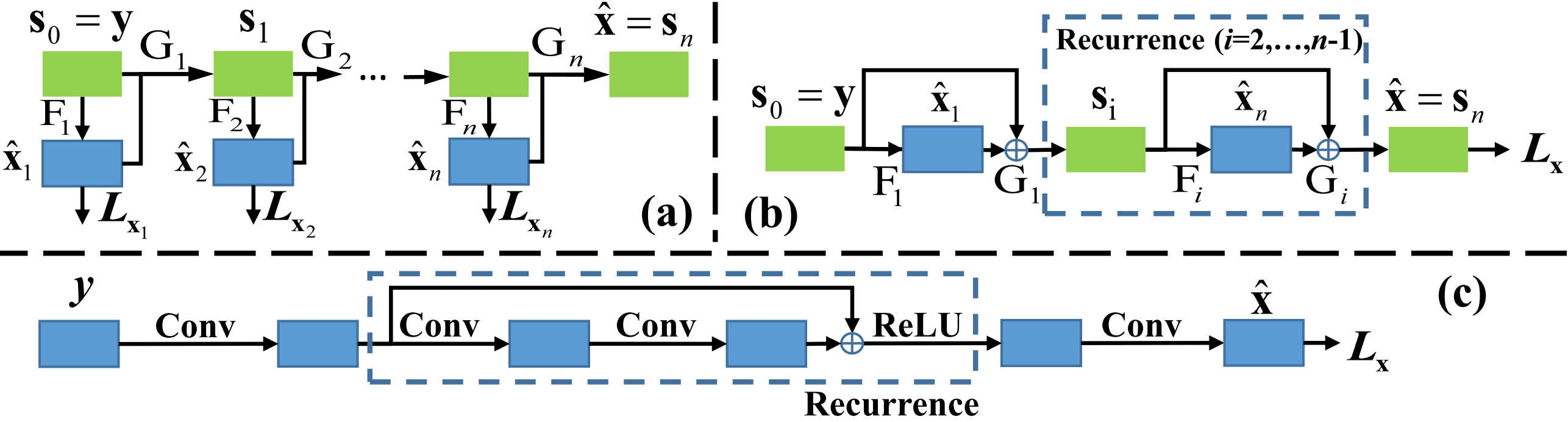
Fig.3. (a) The flowchart of the sub-band reconstruction for image super-resolution. (b) A relaxed version of (a). ${G}_i$ is set as the element-wise summation function. In this framework, only the MSE loss is used to constrain the recovery. (c) The deep network designed with the intuition of (b). ${G}_i$ is the element-wise summation function and ${F}_i$ is modeled by two layer convolutions.
Experimental Results
Datasets. Following the experimental setting in [1] and [2], we compare the proposed method with recent SR methods on three popular benchmark datasets: Set5 [3], Set14 [4] and BSD100 [5] with scaling factors of 2, 3 and 4. The three datasets contain 5, 14 and 100 images respectively. Among them, the Set5 and Set14 datasets are commonly used for evaluating traditional image processing methods, and the BSD100 dataset contains 100 images with diverse natural scenes. We train our model using a training set created in [6], which contains 91 images.
Baseline Methods. We compare our DEGREE SR network (DEGREE) with Bicubic interpolation and the following six state-of-the-art SR methods: ScSR (Sparse coding) [6], A+ (Adjusted Anchored Neighborhood Regression) [7], SRCNN [1], TSE-SR (Transformed Self-Exemplars) [8], CSCN (Deep Sparse Coding) [9] and JSB-NE (Joint Sub-Band Based Neighbor Embedding) [10]. It is worth noting that CSCN and JSB-NE are the most recent deep learning and sub-band recovery based image SR methods respectively.
Our Methods. We use DEGREE-1, DEGREE-2 and DEGREE-MV to
denote three versions of the proposed model when we report
the results. DEGREE-1 has 10 layers and 64 channels, and
DEGREE-2 has 20 layers and 64 channels. The results of
DEGREE-MV are generated by the multi-view testing strategy
via fusing and boosting the results generated by DEGREE-2, similar to CSCN-MV [9] to further investigate the effect
of improving the quality of prior edge maps adopted in
DEGREE on the final performance (see following texts for
more details).
Objective Results.
Table 1. Average PSNR(dB) results of different super-resolution methods on test sets.
| Dataset | Set5 | Set14 | BSD100 | |||||||
|---|---|---|---|---|---|---|---|---|---|---|
| Method | Metric | 2 | 3 | 4 | 2 | 3 | 4 | 2 | 3 | 4 |
| Bicubic | PSNR | 33.66 |
30.39 |
28.42 |
30.13 |
27.47 |
25.95 |
29.55 |
27.2 |
25.96 |
| SSIM | 0.9096 |
0.8682 |
0.8105 |
0.8665 |
0.7722 |
0.7011 |
0.8425 |
0.7382 |
0.6672 |
|
| ScSR | PSNR | 35.78 | 31.34 | 29.07 | 31.64 | 28.19 | 26.4 | 30.77 | 27.72 | 26.61 |
| SSIM | 0.9485 | 0.8869 | 0.8263 | 0.899 | 0.7977 | 0.7218 | 0.8744 | 0.7647 | 0.6983 | |
| A+ | PSNR | 36.56 | 32.6 | 30.3 | 32.14 | 29.07 | 27.28 | 30.78 | 28.18 | 26.77 |
| SSIM | 0.9544 | 0.9088 | 0.8604 | 0.9025 | 0.8171 | 0.7484 | 0.8773 | 0.7808 | 0.7085 | |
| TSE-SR | PSNR | 36.47 | 32.62 | 30.24 | 32.21 | 29.14 | 27.38 | 31.18 | 28.30 | 26.85 |
| SSIM | 0.9535 | 0.9092 | 0.8609 | 0.9033 | 0.8194 | 0.7514 | 0.8855 | 0.7843 | 0.7108 | |
| JSB-NE | PSNR | 36.59 | 32.32 | 30.08 | 32.34 | 28.98 | 27.22 | 31.22 | 28.14 | 26.71 |
| SSIM | 0.9538 | 0.9042 | 0.8508 | 0.9058 | 0.8105 | 0.7393 | 0.8869 | 0.7742 | 0.6978 | |
| CNN | PSNR | 36.34 | 32.39 | 30.09 | 32.18 | 29.00 | 27.20 | 31.11 | 28.20 | 26.70 |
| SSIM | 0.9521 | 0.9033 | 0.853 | 0.9039 | 0.8145 | 0.7413 | 0.8835 | 0.7794 | 0.7018 | |
| CNN-L | PSNR | 36.66 | 32.75 | 30.49 | 32.45 | 29.30 | 27.5 | 31.36 | 28.41 | 26.90 |
| SSIM | 0.9542 | 0.909 | 0.8628 | 0.9067 | 0.8215 | 0.7513 | 0.8879 | 0.7863 | 0.7103 | |
| CSCN | PSNR | 36.88 | 33.10 | 30.86 | 32.50 | 29.42 | 27.64 | 31.40 | 28.50 | 27.03 |
| SSIM | 0.9547 | 0.9144 | 0.8732 | 0.9069 | 0.8238 | 0.7573 | 0.8884 | 0.7885 | 0.7161 | |
| CSCN-MV | PSNR | 37.14 | 33.26 | 31.04 | 32.71 | 29.55 | 27.76 | 31.54 | 28.58 | 27.11 |
| SSIM | 0.9567 | 0.9167 | 0.8775 | 0.9095 | 0.8271 | 0.762 | 0.8908 | 0.791 | 0.7191 | |
| DEGREE-1 | PSNR | 37.29 | 33.29 | 30.88 | 32.87 | 29.53 | 27.69 | 31.66 | 28.59 | 27.06 |
| SSIM | 0.9574 | 0.9164 | 0.8726 | 0.9103 | 0.8265 | 0.7574 | 0.8962 | 0.7916 | 0.7177 | |
| DEGREE-2 | PSNR | 37.40 | 33.39 | 31.03 | 32.96 | 29.61 | 27.73 | 31.73 | 28.63 | 27.07 |
| SSIM | 0.9580 | 0.9182 | 0.8761 | 0.9115 | 0.8275 | 0.7597 | 0.8937 | 0.7921 | 0.7177 | |
| DEGREE-MV | PSNR | 37.61 | 33.70 | 31.30 | 33.11 | 29.77 | 27.92 | 31.84 | 28.76 | 27.18 |
| SSIM | 0.9589 | 0.9212 | 0.8807 | 0.9129 | 0.8309 | 0.7637 | 0.8951 | 0.7956 | 0.7207 | |
| Gain | PSNR | 0.47 | 0.45 | 0.26 | 0.40 | 0.22 | 0.16 | 0.30 | 0.18 | 0.07 |
| SSIM | 0.0022 | 0.0045 | 0.0032 | 0.0034 | 0.0038 | 0.0017 | 0.0043 | 0.0046 | 0.0016 | |
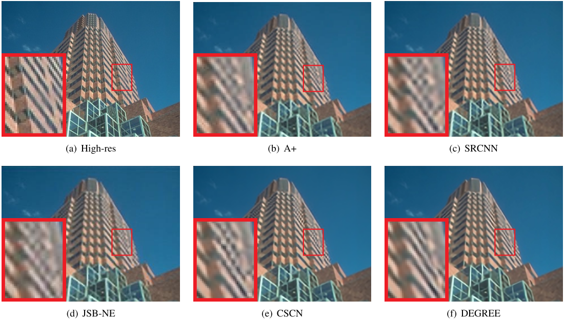
Fig.4. Visual comparisons between different algorithms for the image 86000 (3$\times$). The DEGREE presents less artifacts around the window boundaries.
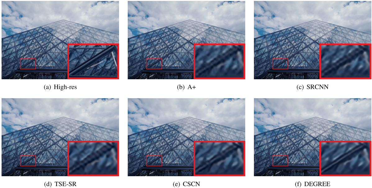
Fig.5. Visual comparisons between different algorithms for the image 223061 (3$\times$). The DEGREE produces more complete and sharper edges.
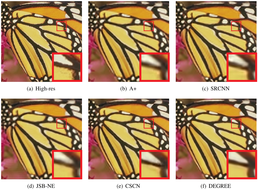
Fig.5. Visual comparisons between different algorithms for the image Butterfly (4$\times$). The DEGREE avoids the artifacts near the corners of the white and yellow plaques, which are present at the results produced by other state-of-the-art methods.
JPEG Artifacts Removal.
Table 1. Comparison of PSNR(dB) and SSIM results of JPEG artifact reduction on CLASSIC5 dataset used in ARCNN, with four QFs (10, 20, 30 and 40). The bold numbers denote the best performance.
| QF | Metric | JPEG | SA-DCT | ARCNN | DEGREE |
|---|---|---|---|---|---|
| 10 | PSNR | 27.82 | 28.88 | 29.04 | 29.36 |
| SSIM | 0.78 | 0.8071 | 0.8111 | 0.8201 | |
| 20 | PSNR | 30.12 | 30.92 | 31.16 | 31.65 |
| SSIM | 0.8541 | 0.8663 | 0.8694 | 0.8777 | |
| 30 | PSNR | 31.48 | 32.14 | 32.52 | 32.92 |
| SSIM | 0.8844 | 0.8914 | 0.8967 | 0.901 | |
| 40 | PSNR | 32.43 | 33 | 33.34 | 33.67 |
| SSIM | 0.9011 | 0.9055 | 0.9101 | 0.9136 |
Table 1. Comparison of PSNR(dB) and SSIM results of JPEG artifact reduction on LIVE1 dataset used in ARCNN, with four QFs (10, 20, 30 and 40). The bold numbers denote the best performance.
| QF | Metric | JPEG | SA-DCT | ARCNN | DEGREE |
|---|---|---|---|---|---|
| 10 | PSNR | 27.82 | 28.88 | 29.04 | 29.22 |
| SSIM | 0.7800 | 0.8071 | 0.8111 | 0.8178 | |
| 20 | PSNR | 30.12 | 30.92 | 31.16 | 31.51 |
| SSIM | 0.8541 | 0.8663 | 0.8694 | 0.8763 | |
| 30 | PSNR | 31.48 | 32.14 | 32.52 | 32.81 |
| SSIM | 0.8844 | 0.8914 | 0.8967 | 0.9002 | |
| 40 | PSNR | 32.43 | 33.00 | 33.34 | 33.60 |
| SSIM | 0.9011 | 0.9055 | 0.9101 | 0.9129 |
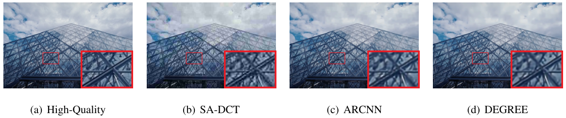
Fig.6. Visual comparisons of JPEG artifacts reduction for the image 223061 in BSD500 (QF: 20). The DEGREE recovers
more straight and long edges.
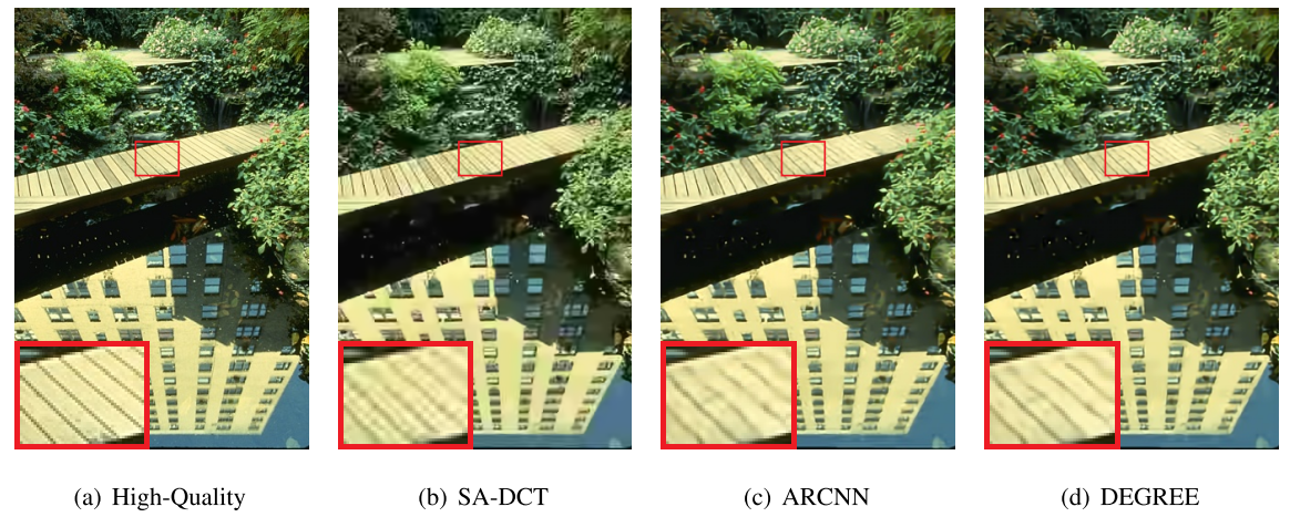
Fig.7.Visual comparisons of JPEG artifacts reduction for the image 148026 in BSD500 (QF: 10). The DEGREE presents
clearer cracks between the boards.
Performance VS Complexity.
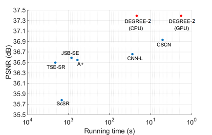 |
Fig.7.The performance comparison between our proposed DEGREE model with state-of-the-art methods, including the final
performance (y-axis) and time complexity (x-axis), in 2$/times$ enlargement on dataset Set5.
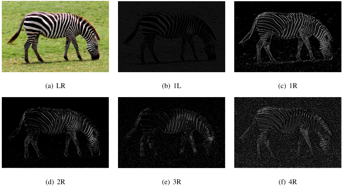
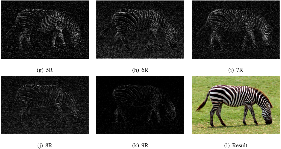
Sub-band Decomposition.
Download and Cite
Download.
More details and results are presented in the following links.
Results
| Data Set \ SF | 2 | 3 | 4 |
| Set5 | Set5_2 | Set5_3 | Set5_4 |
Set14 |
Set14_2 | Set14_3 | Set14_4 |
| BSD300 | BSD300_2 | BSD300_3 | BSD300_4 |
Cite.
@ARTICLE{2016arXivDEGREE,
author = {Wenhan Yang and Jiashi Feng and Fang Zhao and Jiaying Liu and Zongming Guo and Shuicheng Yan},
title = "{Deep Edge Guided Recurrent Residual Learning for Image Super-Resolution}",
journal = {ArXiv e-prints},
eprint = {1604.08671},
year = 2016,
month = Apr,
}
References
[1] Dong, C., Loy, C., He, K., Tang, X., "Image super-resolution using deep convolutional networks", IEEE Transactions on Pattern Analysis and Machine Intelligence, 2015.
[2] Wang, Z., Liu, D., Yang, J., Han, W., Huang, T., "Deep networks for image super-resolution with sparse prior", In: Proc. IEEE Int'l Conf. Computer Vision, June 2015.
[3] M. Bevilacqua, A. Roumy, C. Guillemot and ML. Alberi, "Low-Complexity Single-Image Super-Resolution based on Nonnegative Neighbor Embedding'', BMVC 2012.
[4] Zeyde, R., Elad, M., Protter, M., "On single image scale-up using sparse-representations", In Proceedings of International Conference on Curves and Surfaces, Berlin, Heidelberg, 2012.
[5] D. Martin and C. Fowlkes and D. Tal and J. Malik, "A Database of Human Segmented Natural Images and its Application to Evaluating Segmentation Algorithms andMeasuring Ecological Statistics", in Proc. Int'l Conf. Computer Vision, July, 2001.
[6] Yang, J., Wright, J., Huang, T., Ma, Y., "Image super-resolution via sparse representation", IEEE Transactions on Image Processing, 19(11) , Nov 2010, 2861–2873.
[7] Timofte, R., DeSmet, V., VanGool, L., "A+: Adjusted anchored neigh borhood regression for fast super-resolution", In Proc. IEEE Asia Conf. Computer Vision, 2015.
[8] Huang, J.B., Singh, A., Ahuja, N., "Single image super-resolution from transformed self-exemplars", In Proc. IEEE Int'l Conf. Computer Vision and Pattern Recognition, 2015.
[9] Wang, Z., Liu, D., Yang, J., Han, W., Huang, T., "Deep networks
for image super-resolution with sparse prior", In Proc. IEEE Int'l
Conf. Computer Vision, 2015.
[10] Song, S., Li, Y., Liu, J., Zongming, G., "Joint sub-band based neighbor embedding for image super resolution", In Proc. IEEE Int'l Conf. Acoustics, Speech, and Signal Processing, 2016.