- Mading Li
martinli0822@pku.edu.cn - Jiaying Liu
liujiaying@pku.edu.cn - Jie Ren
renjie@pku.edu.cn - Zongming Guo
guozongming@pku.edu.cn
Published on TCSVT, February 2015 and ISCAS, May 2013.
Overview
Image interpolation is a process that generates high-resolution (HR) images utilizing the information in low-resolution (LR) images. The key task of image interpolation is to estimate the HR pixels interpolated into the LR image. Conventional interpolation algorithms, such as Bilinear and Bicubic interpolations apply a convolution on every interpolated pixel of the HR image. Since these methods apply the same convolution on every pixel, they do not distinguish pixels in plain area and high frequency region. Although these methods have rather low complexity, they produce noticeable reconstruction artifacts near edges and blur the image to some extent.
Since the edge structure is one of the most salient features in natural images, many edge-guided interpolation algorithms are published. One of the most effective method is Autoregressive (AR) Model. An autoregressive (AR) model is a type of random process that is often utilized to model and predict various types of natural signals. It is a set of linear formulas that attempts to obtain an estimation of a system based on the given information. In image processing, every pixel in an image can be estimated by its adjacent neighbors with certain weights. The AR model is defined as follows:
![]()
where ![]() and
and ![]() are the adjacent neighbors and their weights - model parameters - to pixel
are the adjacent neighbors and their weights - model parameters - to pixel ![]() , respectively.
, respectively. ![]() is the estimating error. Based on the assumption that images maintain stability in a local window W, the model parameters can be computed by solving the linear least squares problem showed below,
is the estimating error. Based on the assumption that images maintain stability in a local window W, the model parameters can be computed by solving the linear least squares problem showed below,
![]()
where ![]() consists of pixels in W. The
consists of pixels in W. The ![]() row of
row of ![]() consists of adjacent neighbors of the
consists of adjacent neighbors of the ![]() pixel in
pixel in ![]() . Then unknown pixels in W can be estimated by LR pixels with the same model parameters
. Then unknown pixels in W can be estimated by LR pixels with the same model parameters ![]() .
.
For better estimation, two kinds of AR models in different directions are always applied. One of them uses a pixel's cross-direction adjacent neighbors to estimate it, the other uses its diagonal direction adjacent neighbors. Two sets of weights can be calculated by performing these two AR models in a local window. Therefore, constraints on pixels are stronger, and the unknown pixels can be estimated more precisely.
Li and Orchard [1] proposed a new edge-directed interpolation (NEDI). They computed the parameters of the AR model in the LR image by a least square problem and estimated HR pixels by their neighbor LR pixels using corresponding parameters. Zhang and Wu [2] further proposed a soft-decision adaptive interpolation (SAI) based on NEDI. They added a cross-direction AR model and more correlations between LR pixels and HR pixels. Thus, SAI gained a better performance upon NEDI. However, these algorithms are based on the assumption that the image is piecewise stationary. To account for the fact that natural images are not always stabilized in local windows, our previous work [3] proposed an implicit piecewise autoregressive model-based image interpolation algorithm (IPAR) based on similarity modulated block estimation. In IPAR, a similarity probability model is proposed to model the non-stationarity of image signals.
The General Scale Interpolation
The adaptive algorithms mentioned above have limitation that they can only deal with enlargement whose magnification is two or a power of two. ![]() enlargement is just one of the special circumstances of image enlargement at general scaling factors. In Fig.1, it can be observed that HR pixels and LR pixels have relatively fixed positions in
enlargement is just one of the special circumstances of image enlargement at general scaling factors. In Fig.1, it can be observed that HR pixels and LR pixels have relatively fixed positions in ![]() enlargement (Fig.1(a)). Thus, it is very effective applying AR model in
enlargement (Fig.1(a)). Thus, it is very effective applying AR model in ![]() enlargement. However, such postition is not fixed in more general cases (Fig.1(b) and Fig.1(c)).
enlargement. However, such postition is not fixed in more general cases (Fig.1(b) and Fig.1(c)).
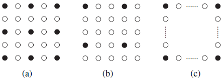
Fig.1. HR pixel and LR pixel in local region at different scaling factors. (a) Scaling factor = 2.0. (b) Scaling factor = 1.5. (c) More general situation.
To solve this problem , we apply two AR models on every pixel in the local window W. Unlike methods for ![]() enlargement, interpolated pixels are estimated by its neighbor pixels no matter what types of pixels they are. The formation is modeled as follows:
enlargement, interpolated pixels are estimated by its neighbor pixels no matter what types of pixels they are. The formation is modeled as follows:
![]()
where vector ![]() consists of pixels in a local window of HR image. Vector
consists of pixels in a local window of HR image. Vector ![]() consists of pixels in the local window excluding the pixels on boundaries of the window.
consists of pixels in the local window excluding the pixels on boundaries of the window. ![]() and
and ![]() are the coefficients that control the weight of two AR models.
are the coefficients that control the weight of two AR models. ![]() and
and ![]() are defined as follow:
are defined as follow:
where ![]() and
and ![]() are the
are the ![]() element of
element of ![]() and
and ![]() ,
, ![]() =(
=(![]() ,
, ![]() ,
, ![]() ,
, ![]() )and
)and ![]() =(
=(![]() ,
, ![]() ,
, ![]() ,
, ![]() ) are the parameters of two AR models, respectively.
) are the parameters of two AR models, respectively.
Since LR pixels are not utilized in AR models, we use these valuable pixels to form a data fidelity term to improve our result. For a local window in HR image, we down-sample it by Bicubic method and compare it to the corresponding window in LR image. The constrain is modeled as follows:
![]()
where vector ![]() consists of pixels in a local window of LR image and matrix
consists of pixels in a local window of LR image and matrix ![]() represents the Bicubic down-sampling process. Obviously, the smaller this constrain's value is, the better estimation we have. Such constrain is useless in
represents the Bicubic down-sampling process. Obviously, the smaller this constrain's value is, the better estimation we have. Such constrain is useless in ![]() enlargement because the pixels that is down-sampled are exactly the same with the corresponding pixels in LR image.
enlargement because the pixels that is down-sampled are exactly the same with the corresponding pixels in LR image.
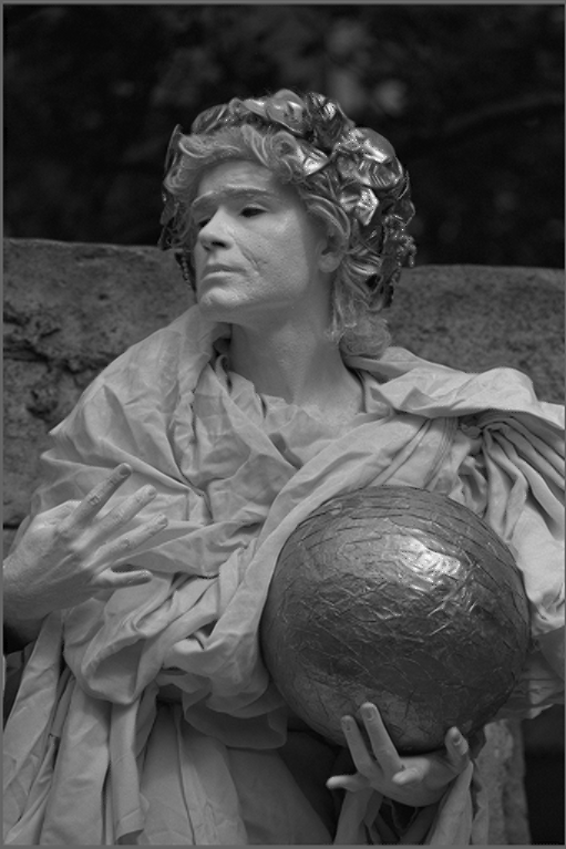
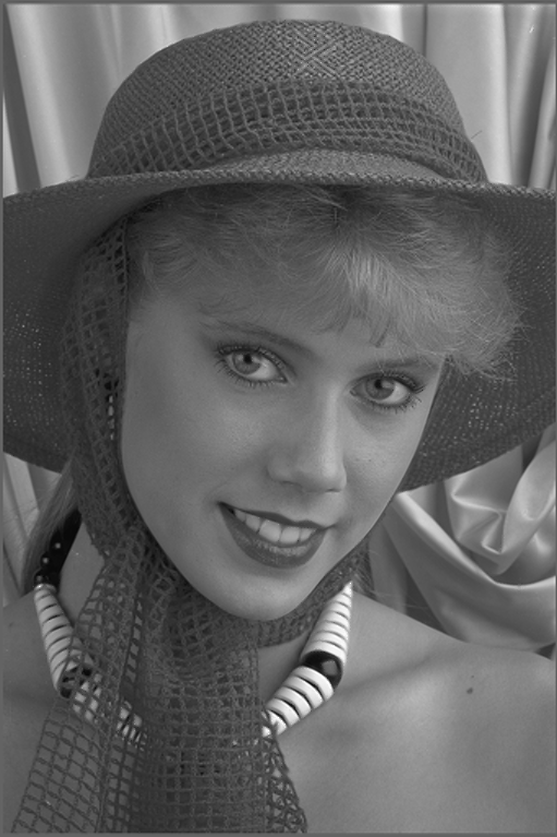
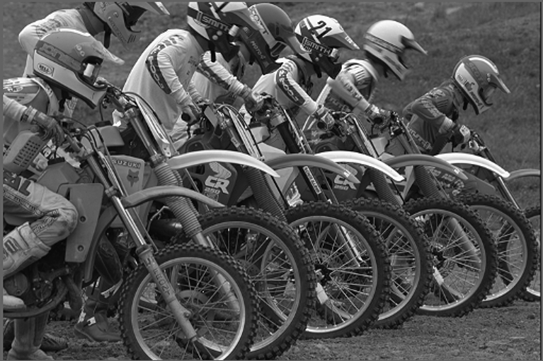
AR model works well when the statistics in the local window are stationary because all AR models of a same type share a same weights in the whole window. However, natural pictures do not maintain stability in most local windows. For example, as illustrated in Fig.2, there are significant differences between an edge-crossing area and a plain area in a local window. Thus, estimations of AR models in this window are not robust. In order to solve this problem, we introduce a method to judge the similarity between the pixel to-be-output (usually the center pixel) and other pixels in the local window.
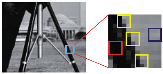
Fig.2. Similar patches in local window. Patches in yellow frames are similar to each other but different from those in red or navy blue.
Naturally we prefer to give more weight on the pixel (in other words, its corresponding AR model) that are more similar to the center pixel, and vice versa. It is commonly agreed that pixels are similar if there is a small difference between their local structures. Moreover, two pixels are likely to be similar if they are close to each other. Thus, the weight is a composite of two parts. One of them is the similarity of two center pixels' local structures. The other is the distance between them. The weight ![]() between two pixels
between two pixels ![]() and
and ![]() is defined as
is defined as
![]()
where ![]() represents the similarity of two center pixels' local structures.
represents the similarity of two center pixels' local structures. ![]() represents the degree of two pixels' distance. They are described as
represents the degree of two pixels' distance. They are described as
![]()
![]()
where ![]() and
and ![]() represent vectors consisting of the 8-connected neighborhood of
represent vectors consisting of the 8-connected neighborhood of ![]() and
and ![]() , respectively;
, respectively; ![]() and
and ![]() are the spatial coordinates of
are the spatial coordinates of ![]() and
and ![]() , respectively.
, respectively. ![]() and
and ![]() control the shape of the exponential function.
control the shape of the exponential function.
After obtaining all pixels' weight to the center pixel, we can form a diagonal weight matrix ![]() which represents the weight distribution in current local window. By adding the weight matrix
which represents the weight distribution in current local window. By adding the weight matrix ![]() , we can get the objective function described below,
, we can get the objective function described below,
![]()
For simple representation, the objective function can be represented by a least square problem as
![]()
where is the residue vector, representing the estimating residue. It is described as
=.gif)
The least square problem can be linearized by adding ![]() ,
, ![]() and
and ![]() as
as
where ![]() and
and ![]() are constructed as follows: the
are constructed as follows: the ![]() row of
row of ![]() is a vector constructed by four diagonal neighbors of pixel
is a vector constructed by four diagonal neighbors of pixel ![]() . The
. The ![]() row of
row of ![]() is a vector constructed by four cross-direction neighbors of pixel
is a vector constructed by four cross-direction neighbors of pixel ![]() .
.
For simple representation, the linearized function can be written as follows:
![]()
where
Therefore, given the initial values of ![]() ,
, ![]() and
and ![]() , we can obtain
, we can obtain ![]() and use it to update
and use it to update ![]() ,
, ![]() and
and ![]() for the next iteration. In our implementation, we use Bicubic's result as the initial value of
for the next iteration. In our implementation, we use Bicubic's result as the initial value of ![]() ,
, ![]() and
and ![]() are initialized as (1/4, 1/4, 1/4, 1/4).
are initialized as (1/4, 1/4, 1/4, 1/4).
In order to alleviate the complexity of the proposed method, we only apply the proposed algorithm on high-frequency areas. Furthermore, we output the center ![]() pixels at once. It may slightly reduce the performance, but can lead to a 9 times speed-up. Meanwhile, in order to avoid blocking artifacts, we produce an overlapping region between adjacent windows and the offset is set to be 3 pixels. In Fig.3, the output pixels of two adjacent windows are shown. It can be seen that every pixel except for the pixels in boundary areas of the whole image can be processed.
pixels at once. It may slightly reduce the performance, but can lead to a 9 times speed-up. Meanwhile, in order to avoid blocking artifacts, we produce an overlapping region between adjacent windows and the offset is set to be 3 pixels. In Fig.3, the output pixels of two adjacent windows are shown. It can be seen that every pixel except for the pixels in boundary areas of the whole image can be processed.
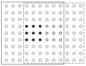
Fig.3. Possible configuration used in proposed algorithm. The size of windows is set to be ![]() . The square in full line represents the current window while the square in dashed line represents its next window. Black pixels and gray pixels are the output of the current window and the next window, respectively.
. The square in full line represents the current window while the square in dashed line represents its next window. Black pixels and gray pixels are the output of the current window and the next window, respectively.
Experimental results
Experiment 1.1 (scaling factor = 1.5)
| Images | Bicubic | Wu[4] | Proposed |
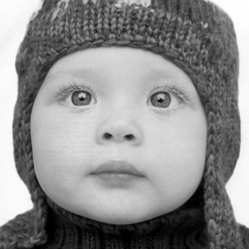
| Child | 39.10 | 37.32 | 39.20 |
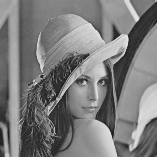
| Lena | 37.67 | 35.61 | 38.29 |
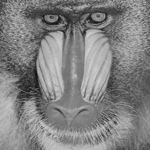
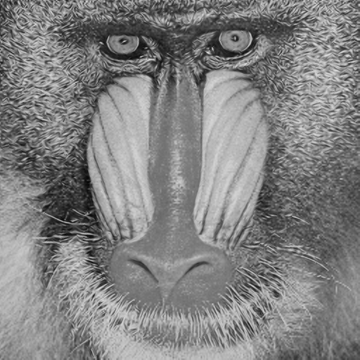
| Baboon | 26.19 | 24.72 | 26.50 |
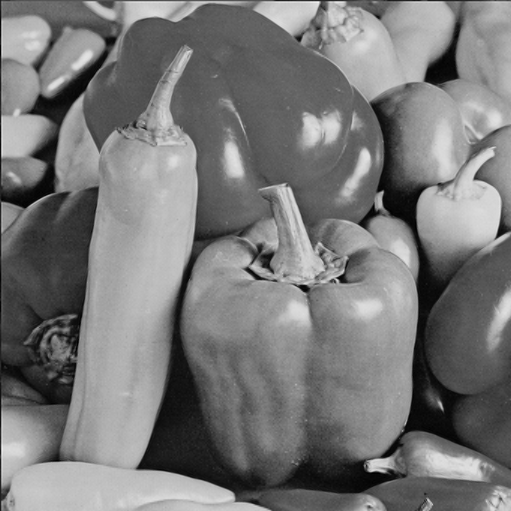
| Pepper | 35.58 | 34.53 | 36.09 |
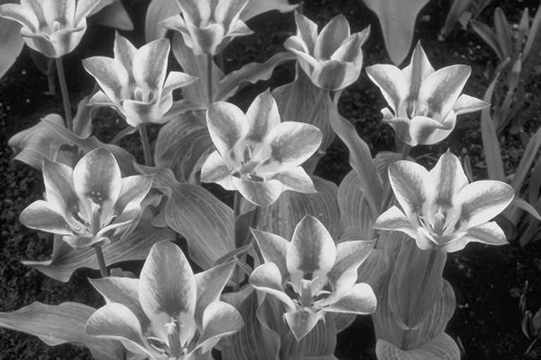
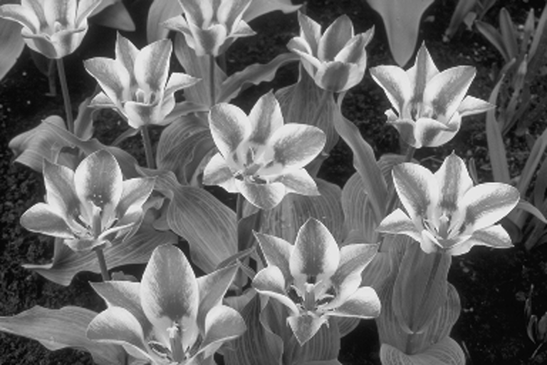
| Tulip | 38.23 | 35.32 | 39.95 |
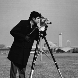
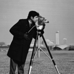
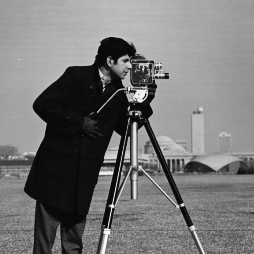
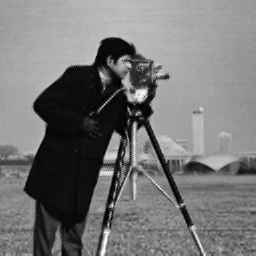
| Cameraman | 29.20 | 27.42 | 30.37 |
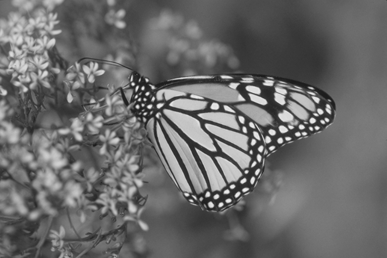
| Monarch | 36.06 | 32.62 | 37.06 |
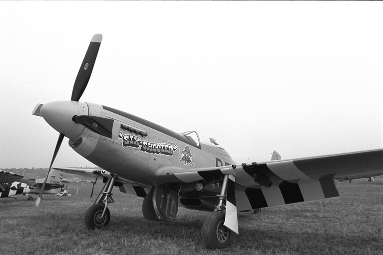
| Airplane | 34.29 | 32.51 | 35.25 |
| Caps | 37.40 | 36.34 | 38.08 |
| Statue | 34.90 | 32.87 | 35.35 |
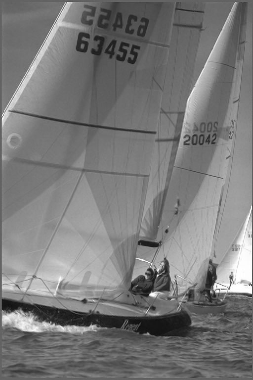
| Sailboat | 35.52 | 34.13 | 36.86 |
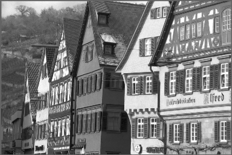
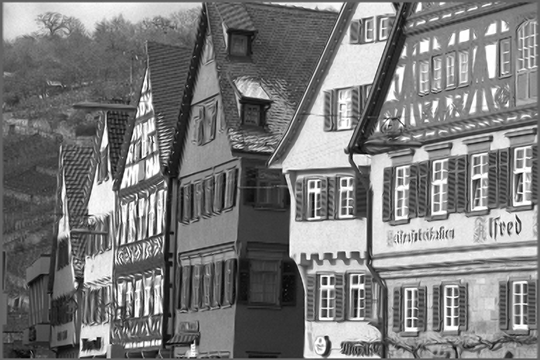
| House | 26.23 | 23.60 | 27.00 |
| Woman | 36.85 | 35.71 | 37.13 |
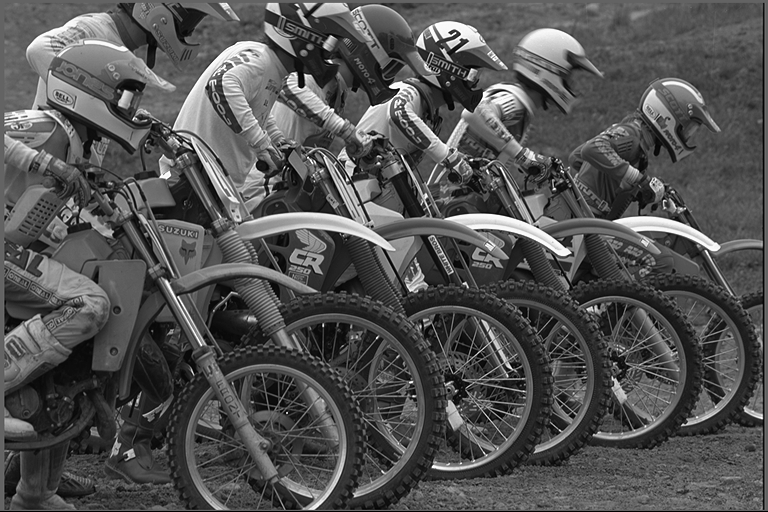
| Bike | 29.94 | 27.57 | 31.26 |
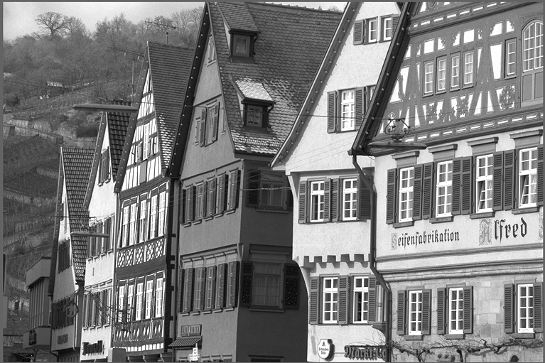
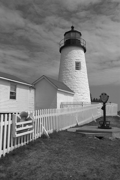
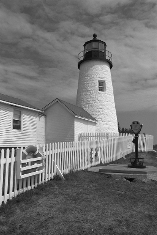
| Lighthouse | 30.83 | 28.81 | 31.88 |
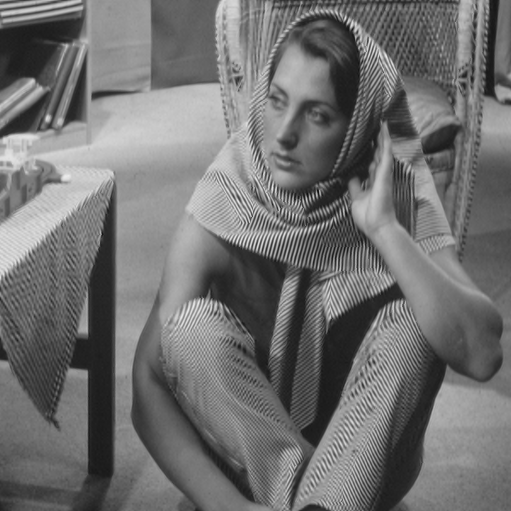
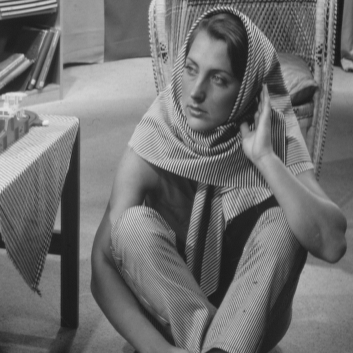
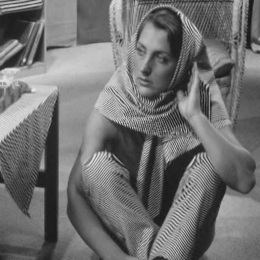
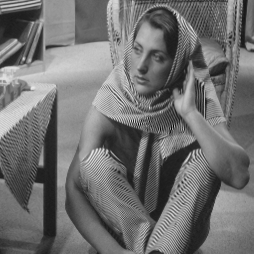
| Barbara | 28.02 | 27.30 | 26.77 |
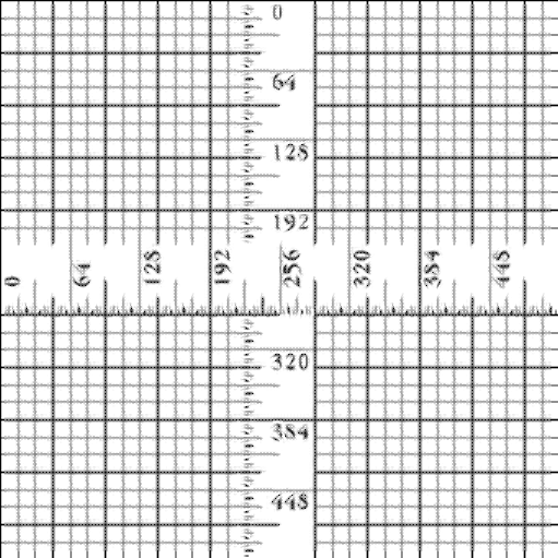
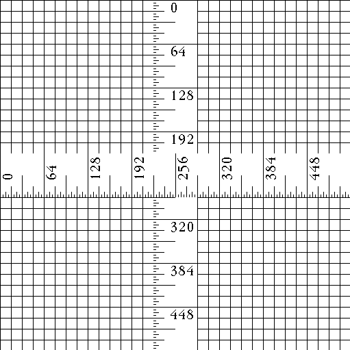
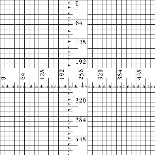
| Ruler | 13.85 | 12.30 | 14.18 |
| Slope | 29.10 | 28.24 | 29.52 |
| Average | 32.16 | 30.38 | 32.82 |
Experiment 1.2 (scaling factor = 1.5)
We test our algorithm on the first 15 frames of each sequence.
| Sequences | JSVM [5] | Bicubic | Proposed |
| akiyo | 39.50 | 41.79 | 43.81 |
| foreman | 39.60 | 42.17 | 43.94 |
| highway | 40.85 | 43.07 | 45.70 |
| Average | 39.99 | 42.34 | 44.48 |
Experiment 2 (scaling factor = 1.7)
| Images | Bicubic | Wu[4] | Proposed |
| Child | 37.62 | 36.23 | 37.68 |
| Lena | 36.26 | 34.64 | 36.78 |
| Baboon | 24.92 | 23.92 | 25.01 |
| Pepper | 34.30 | 33.51 | 34.79 |
| Tulip | 36.29 | 34.23 | 37.96 |
| Cameraman | 27.64 | 26.39 | 28.68 |
| Monarch | 34.27 | 31.72 | 35.20 |
| Airplane | 32.68 | 31.49 | 33.38 |
| Caps | 35.84 | 35.16 | 36.42 |
| Statue | 33.43 | 31.92 | 33.53 |
| Sailboat | 33.80 | 32.98 | 34.93 |
| House | 24.68 | 22.73 | 24.99 |
| Woman | 35.25 | 34.52 | 35.44 |
| Bike | 28.33 | 26.72 | 29.45 |
| Lighthouse | 29.22 | 27.64 | 29.80 |
| Barbara | 26.54 | 25.70 | 25.59 |
| Ruler | 12.83 | 11.73 | 12.95 |
| Slope | 30.38 | 28.58 | 30.75 |
| Average | 30.79 | 29.44 | 31.30 |
Experiment 3 (scaling factor = 2)
| Images | Bicubic | NEDI [1] | SAI[2] | IPAR[3] | JSVM[5] | Wu [4] | Proposed |
| Child | 35.49 | 34.56 | 35.63 | 35.70 | 31.81 | 35.02 | 35.49 |
| Lena | 34.01 | 33.72 | 34.76 | 34.79 | 30.07 | 33.66 | 34.49 |
| Baboon | 22.47 | 22.55 | 22.70 | 22.69 | 21.24 | 22.55 | 22.37 |
| Pepper | 32.06 | 29.32 | 31.84 | 32.69 | 28.41 | 32.15 | 32.56 |
| Tulip | 33.82 | 33.76 | 35.71 | 35.85 | 29.37 | 33.60 | 35.26 |
| Cameraman | 25.51 | 25.44 | 25.99 | 26.06 | 23.63 | 25.49 | 25.55 |
| Monarch | 31.93 | 31.80 | 33.08 | 33.34 | 28.47 | 31.31 | 32.87 |
| Airplane | 29.40 | 28.00 | 29.62 | 30.05 | 26.92 | 29.47 | 29.87 |
| Caps | 31.25 | 31.19 | 31.64 | 31.67 | 30.06 | 31.33 | 31.53 |
| Statue | 31.36 | 31.01 | 31.78 | 31.94 | 29.04 | 31.16 | 31.35 |
| Sailboat | 30.12 | 30.18 | 30.69 | 30.85 | 28.12 | 30.31 | 30.39 |
| House | 22.20 | 21.74 | 22.28 | 22.33 | 20.28 | 21.75 | 22.10 |
| Woman | 31.17 | 30.73 | 31.27 | 31.34 | 29.62 | 31.08 | 31.26 |
| Bike | 25.41 | 25.25 | 26.28 | 26.31 | 23.35 | 25.39 | 25.85 |
| Lighthouse | 26.97 | 26.37 | 26.70 | 26.76 | 25.09 | 26.46 | 27.13 |
| Barbara | 24.46 | 22.36 | 23.55 | 23.10 | 23.18 | 23.85 | 23.26 |
| Ruler | 11.98 | 11.49 | 11.37 | 11.81 | 10.43 | 12.24 | 12.50 |
| Slope | 26.74 | 26.54 | 26.63 | 26.78 | 24.48 | 26.87 | 27.84 |
| Average | 28.13 | 27.56 | 28.42 | 28.56 | 25.75 | 27.98 | 28.43 |
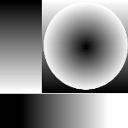
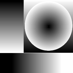
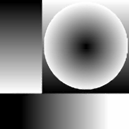
Experiment 4 (model weights)
![]() and
and ![]() represent the weights of two autoregressive (diagonal direction and cross direction). Each point
(x, y) represent the PSNR of the result when
represent the weights of two autoregressive (diagonal direction and cross direction). Each point
(x, y) represent the PSNR of the result when ![]() is set to be x and
is set to be x and ![]() is set to be y. The more red the color is, the corresponding PSNR value is higher; the more blue the color is, the corresponding PSNR value is lower.
is set to be y. The more red the color is, the corresponding PSNR value is higher; the more blue the color is, the corresponding PSNR value is lower.
airplane

cameraman

Notes
(1) The Bicubic method is labeled as "BC";
(2) The new edge-directed interpolation method in [1] is labeled as "NEDI";
(3) Thw soft-decision and adaptive interpolation in [2] is labeled as "SAI";
(4) The implicit piecewise autoregressive mode based image interpolation in [3] is labeled as "IPAR";
(5) The adaptive resolution upconversion algorithm in [4] is labeled as "Wu";
(6) The spatial scalability extension in [5] is labeled as "JSVM";
(7) The proposed method is labeled as "AGSI";
(8) The original image is labeled as "HR";
References
[1] X. Li and M.T. Orchard, “New edge-directed interpolation,” IEEE Trans. Image Processing, vol. 10, no. 10, pp. 1521–1527, October 2001.
[2] X. Zhang and X. Wu, “Image interpolation by adaptive 2-d autoregressive modeling and soft-decision estimation,” IEEE Trans. Image Processing, vol. 17, no. 6, pp. 887–896, June 2008.
[3] J. Ren, J. Liu, W. Bai, Z. Guo, "Similarity modulated block estimation for image interpolation." IEEE International Conference on Image Processing, 2011.
[4] X. Wu, M. Shao, X. Zhang, "Improvement of H.264 SVC by model-based adaptive resolution upconversion", IEEE International Conference on Image Processing, 2010
[5] A. Segall and G. Sullivan, "Spatial Scalability Within the H.264/AVC Scalable Video Coding Extension", IEEE Transactions on Circuits and Systems for Video Technology, vol.17, no.9, pp.1121-1135, 2007