Image Super-Resolution using Saliency-based Context-Aware
Sparse Decomposition
Wei Bai,
Saboya Yang,
Jiaying Liu,
Jie Ren,
Zongming Guo
(click to contact us)
Published on VCIP, November 2013.
Introduction
Sparse representation of signals on over-complete dictionaries is a rapidly evolving field. The basic model suggests that natural signals can be compactly expressed as a linear combination of prespecified atom signals, where the linear coefficients are sparse (i.e., most of them zeros). Formally, let $x\in{\mathbb{R}^{n}}$ be a column signal, and $D\in{\mathbb{R}^{n\times{m}}}$ be a dictionary, the sparsity assumption is described by the following sparse approximation problem: \begin{equation} \label{eq:sparserepre} x\approx{D\gamma},~~s.t. \|\gamma\|_{0}\leq\epsilon. \end{equation} where $\gamma$ is the sparse representation of $x$, $\epsilon$ is a predefined threshold. The $l_{0}$-norm $\|\cdot\|_{0}$ counts the nonzero entries of a vector, claiming the sparsity of $x$. Though $l_{0}$-norm optimization is a NP-hard problem, there are various ways to solve it [1,2].
Sparse representation-based super-resolution (SR) techniques are extensively studied in recent years. They attempt to capture the co-occurrence prior between low-resolution (LR) and high-resolution (HR) image patches. Yang et al. [3] used a coupled dictionary learning model for image super-resolution. They assumed that there exist coupled dictionaries of HR and LR images, which have the same sparse representation for each pair of HR and LR patches. After learning the coupled dictionary pair, the HR patch is reconstructed on HR dictionary with sparse coefficients coded by LR image patch over the LR dictionary. In this typical framework of sparse representation-based SR method, the dictionary is determined on a general training set and the prior model to constrain the restoration problem is the sparsity of each local patch.
In this paper, we present a novel saliency-modulated context-aware sparse decomposition method for image super resolution. Similar images are obtained from the Internet by content-based image retrieval to build a specialized database. Then example patches from the salient regions of the database are extracted to train a salient dictionary, which is especially adaptive to local structures. In addition, to better explore the correlations among patches, we apply context-aware sparse decomposition to salient regions based on the observation that salient regions tend to be more structured.
Saliency-Modulated Context-Aware Sparse Decomposition
Conventional methods randomly choose patches to build training set $X$, which results in a general dictionary. But for a particular LR image, this dictionary is too general to express certain structural details. We improve the dictionary learning model from two levels to enhance the adaptiveness of learned dictionaries. First, similar images of the LR image are gathered to be candidate training set. Then, we go on to narrow it down to salient parts of images in the training set. The proposed dictionary training scheme is based on two facts: 1) Similar images contain more useful information than general images that will help compensate for the LR image. 2) Salient regions are highly structured, signals extracted from the salient regions should be closely correlated. So the learned dictionary is especially adaptive to the structure of the salient regions. Since attended salient regions need to be treated with more acuity from the human visual perspective, we apply salient dictionaries only to salient regions. For the less attended non-salient regions, a general dictionary will do.
In the sparse coding phase, sparsity of each independent patches is used to regularize the optimization problem. In other words, each patch is sparsely coded independently and overlapped regions are averaged to keep smoothness along boundaries. However, neighboring patches are closely correlated. They may tend to have similar sparse codes. Especially for patches in salient regions, the highly structured property makes them more dependent on each other. Thus we introduce the context-aware sparse decomposition to employ the dependencies between the dictionary atoms used to decompose the patches. Such improvement on the prior model imposes more constraints on the restoration problem, which will help preserve more structural details.
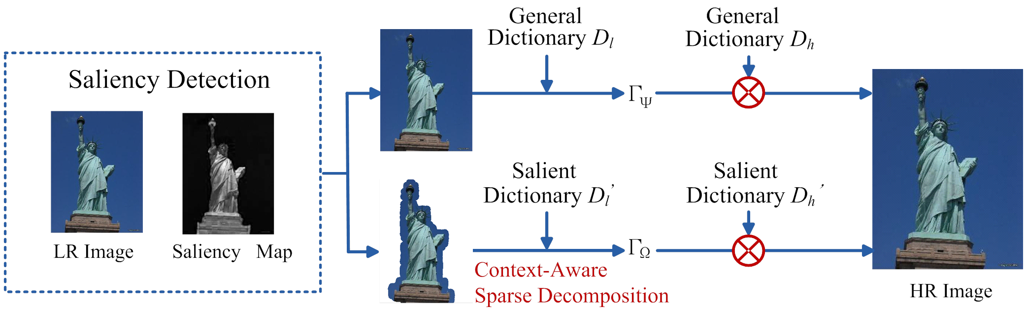
Fig. 1. Flow diagram of the proposed algorithm.
Based on the characteristics of saliency, the proposed algorithm generates adaptive dictionaries and also sparsely decompose patches in a correlated way. A set of similar images to the LR image are collected in $\Psi$, and then comes the salient database $\Omega$. Obviously, $\Omega\subseteq\Psi$. Let $X_{\Psi}$ be a set of patches which are extracted from the whole images in the database, and $X_{\Omega}$ be the patches extracted from the salient regions in the images of the database. Then the general dictionary, $\{D_l$, $D_h\}$, and the saliency-modulated dictionary, $\{D^{'}_l, D^{'}_h\}$, are obtained by training on $X_{\Psi}$ and $X_{\Omega}$. $\Gamma_\Psi$ and $\Gamma_\Omega$ are sparse codes for non-salient and salient regions, as Fig.1 illustrates. Note that, $\Gamma_\Omega$ is obtained by context-aware sparse coding. Therefore, salient regions are reconstructed with more accuracy owing to the context-aware sparse coding process.
Instead of enforcing the compatibility of overlapped regions between neighboring patches, we investigated the context-aware sparse decomposition of patches, which means the correlations between the structural information of the whole patches, not only in the overlapped regions, are explored. Correlations between the structural components of the adjacent patches refer to the dependencies between the dictionary atoms which are used to decompose the patches. As mentioned before, regions that are salient to human eyes tend to be highly structured and probably share similar sparse codes. This provides a reasonable scenario to apply the context-aware sparse decomposition.
Let $\gamma_{i}$ be the sparse representation vector of patch $x_{i}$, and $\gamma_{i\diamond{t}}, t=1,2,...8,$ be the sparse codes of $x_{i}$'s neighbor patches in 8 directions (see Fig.2, e.g., the patch in dash line stands for direction-1 patch). Denote $S_{i}$ as sparsity pattern of representation $\gamma_{i}$ ($S_i\in{\{-1,1\}^{m}}$), if $\gamma_{i}(j)\neq{0}$ (i.e., the j-th atom of $\gamma_{i}$) then $S_{i}(j)=1$, otherwise $S_{i}(j)=-1$. $S_{i\diamond{t}}$ represents the sparsity pattern of the adjacent patch in orientation $t$.

Fig. 2. The local neighborhood system of patch $x_{i}$ with a spatial configuration of eight different orientations.
Given all the orientated neighboring sparsity patterns $\{S_{\diamond{t}}\}_{t=1}^{T}$, we define the context-aware energy $E_{c}(S)$ by \begin{equation} \label{eq:CATerm} E_{c}(S)=-\sum_{t=1}^{T}S^{T}W_{\diamond{t}}S_{\diamond{t}}, \end{equation} $W_{\diamond{t}}$ captures the interaction strength between dictionary atoms in orientation $t$. For instance, to the current patch $x_{i}$, $W_{\diamond{t}}(m,n)=0$ indicates $S_{i}(m)$ and $S_{i\diamond{t}}(n)$ tend to be independent; $W_{\diamond{t}}(m,n)>0$ indicates $S_{i}(m)$ and $S_{i\diamond{t}}(n)$ tend to be activated simultaneously; $W_{\diamond{t}}(m,n)<0$ indicates $S_{i}(m)$ and $S_{i\diamond{t}}(n)$ tend to be mutually exclusive. We will introduce how to compute $W_{\diamond{t}}$ later in this section.
Meanwhile, the sparsity penalty energy $E_{s}(S)$ is taken into account: \begin{equation} \label{eq:SparsityTerm} E_{s}(S)=-S^{T}b, \end{equation} where $b=[b_{1},b_{2},...,b_{m}]^{T}$ is a vector of model parameters, and $b_{i}$ is associated with the dictionary atom, $b_{i}<0$ favors $S_{i}=-1$. The total energy for each sparsity pattern is the sum of the context-aware energy and the sparsity energy, i.e., $E_{total}=E_{c}(S)+E_{s}(S)$. The prior probability can then be formalized using the total energy, \begin{equation} \label{eq:TotalTerm} \begin{aligned} \Pr(S) \propto &\exp\left({-E_{total}}\right) \\ \propto &\exp\left(S^T \left(\sum_{t=1}^T{W_{\diamond{t}}S_{\diamond{t}}}+b \right)\right). \end{aligned} \end{equation} Let $\tilde{W} = \left[W_{\diamond1},\dots,W_{\diamond J}\right]$, and $\displaystyle\tilde{S} = \left[(S_{\diamond1})^T,\dots,(S_{\diamond J})^T\right]^T$, then eq.(\ref{eq:TotalTerm}) can be expressed in a clearer form, \begin{equation}\label{eqn:ContextPrior2} \Pr(S) = \frac{1}{Z(\tilde{W},b)}\exp\left(S^T\left({\tilde{W}\tilde{S}}+b\right)\right), \end{equation} where $\tilde{W}$, $b$ are model parameters, and $Z(\tilde{W},b)$ is the function for normalization. It shows compared with conventional sparsity priors, the proposed prior model places more emphasis on the dependencies of atoms in the spatial context.
For the above new prior, the model parameters including $\tilde{W}, b,$ and $\{\sigma_{\gamma,i}^2\}_{i=1}^m$ should be estimated. $\sigma_{\gamma,i}^2$ stands for variance of each nonzero coefficient $\gamma_i$. Given $\mathcal{X} = \{x^k,S^k,\gamma^k, \tilde{S}^k\}_{k=1}^{K}$ as examples sampled from the model, we suggest using the Maximum Likelihood Estimation (MLE) for learning the model parameters ${\theta}=[\tilde{W}, b, \{\sigma_{\gamma,i}^2\}_{i=1}^m] \in \Theta$. Mathematically, we have \begin{equation} \begin{aligned} \hat{\theta}_{ML} &= \arg\max_{\theta}\Pr\left(\mathcal{X}|\theta\right) =\arg\max_{\theta}\sum_{i=1}^m\mathcal{L}(\sigma_{\gamma,i}^2) + \mathcal{L}(\tilde{W},b), \end{aligned} \end{equation} where \begin{equation} \begin{aligned} \mathcal{L}(\sigma_{\gamma,i}^2) &= \frac{1}{2}\sum_{k=1}^K{f^k_i},\\ \mathcal{L}(\tilde{W},b) &= \frac{1}{2}\sum_{k=1}^K\left(S^k\right)^T\left(\tilde{W}\tilde{S}^k + b\right) - K\ln Z(\tilde{W},b), \end{aligned} \end{equation} are log-likelihood functions for the model parameters and \begin{equation} f^k_i = \begin{cases} \cfrac{\left(\gamma_i^{k}\right)^2}{{\sigma_{\gamma,i}^2}} + \ln({\sigma_{\gamma,i}^2}), & S_i^k = 1,\\ 0, & S_i^k=-1.\end{cases} \end{equation}
For the estimation of variances, a closed-form estimator is obtained by: \begin{equation} \hat{\sigma}_{\gamma,i}^2 = \frac{\sum_{k=1}^{K}{(\gamma_i^{k})^2 \cdot q_i^k}}{\sum_{k=1}^{K}{q_i^k}}, \end{equation} where $$q_i^k = \begin{cases} 1, & S^k_i=1, \\ 0, & S^k_i=-1.\end{cases}$$
However, ML estimation of $\tilde{W}$ and $b$ is computationally intensive due to the exponential complexity in $m$ associated with the partition function $Z(\tilde{W},b)$. We adopted an efficient algorithm [4] using the MPL estimation and sequential subspace optimization (SESOP) method to tackle the problem.
Experimental Results
| Images | Bicubic | ScSR [1] | Salient OMP | Proposed |
| Liberty | 23.03 | 23.50 | 23.57 | 23.60 |
| Horse | 27.61 | 27.92 | 28.11 | 28.13 |
| Colosseum | 22.21 | 22.70 | 22.79 | 22.81 |
| Tower | 29.52 | 29.95 | 30.08 | 30.09 |
| Average | 25.59 | 26.01 | 26.14 | 26.16 |
Reference
[1] K. Engan, S. Ease, and J. Husoy, “Multi-frame compression: Theory and design,” Signal Processing, vol. 80, no. 10, pp. 2121–2140, Oct. 2000.
[2] M. Aharon, M. Elad, and A. Bruckstein, “K-svd: An algorithm for designing overcomplete dictionaries for sparse representation,” IEEE Transactions on Signal Processing, vol. 54, no. 11, pp. 4311–4322, Nov. 2006.
[3] J. Yang, J. Wright, T. Huang, and Y. Ma, “Image super-resolution via sparse representation,” IEEE Transactions on Image Processing, vol. 19, no. 11, pp. 2861–2873, Nov. 2010.
[4] A. Hyvarinen, “Consistency of pseudolikelihood estimation of fully visible boltzmann machines,” Neural Computation, vol. 18, no. 10, pp. 2283–2292, 2006.