- Jie Ren
renjie@pku.edu.cn - Jiaying Liu
liujiaying@pku.edu.cn - Wei Bai
janelle@pku.edu.cn - Zongming Guo
guozongming@pku.edu.cn
Publication Bibtex
@INPROCEEDINGS{RLB+2011,
author = {Jie Ren, and Jiaying Liu, and Wei Bai, and Zongming Guo},
title = {Similarity Modulated Block Estimation for Image Interpolation},
booktitle = {Image Processing (ICIP), 2011 18th IEEE International Conference
on},
year = {2011} }
@ARTICLE{RLB+2011a,
author = {Jie Ren, and Jiaying Liu, and Wei Bai, and Zongming Guo},
title = {Implicit Piecewise Autoregressive Model-Based Image Interpolation
Algorithm},
journal = {Accepted by Journal of Software (JOS)},
year = {2011},
volume = {99},
pages = {1-1} }
Published on JOS, May 2012 and ICIP, September 2011.
Overview
Image interpolation is the process of producing high-resolution (HR) images from its low-resolution (LR) counterparts. Understanding and modeling the inherent image structures partly reflected by LR images is the key task and challenge for image interpolation. Conventional interpolation methods, such as bilinear and bicubic interpolation regard the ground-truth HR images to be continuous and smooth. These methods work well in smooth regions but fail to capture the fast varying property around edge structures, suffering from the problem of aliasing, blurring or ringing artifacts.
To address the problems of conventional interpolation methods, many spatial adaptive interpolation methods have been proposed to preferably preserve the edge structures. A major challenge for developing such adaptive interpolation algorithm is modeling the nonstationarity of image signals, in particular the edge structures. Some explicite edge-adaptive methods extract the edge structural information, such as edge directions and widths, and then fitted the missing pixels by directional interpolating along the detected edge directions. These methods in practical are difficult to carry out when irregular textures and noise are present in the LR images.
In contrasty, implicit methods like the Auto-Regression (AR) model estimate the edge information using the local stationary statistics. A 2-D image signal can be modeled as AR process as follows:
where  are the model parameters,
  is a white noise, and
  is a local neighborhood around the pixel
  . The number of neighbors in decides the order of the model. The model parameters should be adaptive to the local image structures. So it is estimated by the samples within a local window centered at pixel . However, the fixed size of local window can not adapt to the local edge features at different scales.
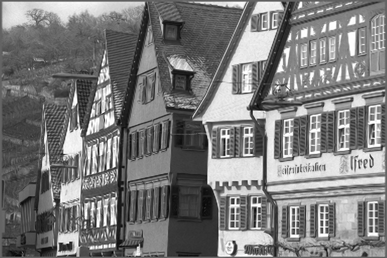
Especially when the scale of local edge feature is smaller than
the selected local window size, the stationarity assumption is
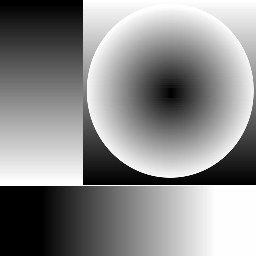
violated. Fig. 1 is an example for the above analysis.
. The number of neighbors in decides the order of the model. The model parameters should be adaptive to the local image structures. So it is estimated by the samples within a local window centered at pixel . However, the fixed size of local window can not adapt to the local edge features at different scales.
Especially when the scale of local edge feature is smaller than
the selected local window size, the stationarity assumption is
violated. Fig. 1 is an example for the above analysis.

Fig. 1. Illustration of a local window and the irregularity of statistics stationary. To estimate the optimal model parameters at center pixel yc, sample pixels are assigned different weights to indicate the similarity probability in statistics.
We propose to probabilistic modeling the stationary area within the local window. Then each pixel  has a probability
  to indicate the consistency to the AR model parameters of the center pixel . Then a block of pixels within the local window W are jointly estimated by minimizing the following energy function:

 is a parameter to balance the energy functions of
  and
and  , which are fitting errors of diagonal AR model and cross-directional AR model, respectively.
 and
and  are the parameters of diagonal and cross-directional AR model, respectively.
  and
and  are the diagonal and cross-direction neighbors. The spatial configurations of these two AR models are illustrated in Fig. 2.
 |
 |
 |
 |
| (a) | (b)> | (c)> | >(d) |
Fig.2 The spatial configuration of AR models. (a), (b) illustrate the diagonal relationship. (c), (d) illustrate the cross-direction relationship for HR and LR pixels.
Implementation
The similarity probability for each pixel represents the degree of local structural similarity between two pixels in a local window W. The local pixel structure are represented by its diagonal neighbors as in Fig.3(a).
 |
 |
| (a) | (b) |
Fig.3. Illustration of similarity probability modeling. (a)Local pixel structure representation (b)An example of similarity probability distribution in a local window(yellow rectangle).
Then the similarity probability between two pixels and  can be calculated by:

where  is the vector containing the diagonal pixel neighbors.
  is the pixel intensity of and
  is the position vector of . The parameters
  are set to 17, 50000, 33 respectively to obtain the best performance.
After introducing the similarity probability modeling, interpolation of high-resolution missing pixels can be solved by minimizing the energy function described above:

The model parameters , and the missing HR pixels  are both treated as variables in the non-linear optimal estimation. Iterative methods, such as gradient descent, are needed to solve the optimization.
To reduce the computational cost, the parameters , can be approximately estimated by the available LR pixels
are both treated as variables in the non-linear optimal estimation. Iterative methods, such as gradient descent, are needed to solve the optimization.
To reduce the computational cost, the parameters , can be approximately estimated by the available LR pixels  in local window W ahead of time,

where  is the diagonal neighbor pixels on the LR image grid (Please refer to the graphical illustration in Fig.2).
This approximation reduces the problem to a linear estimation,
is the diagonal neighbor pixels on the LR image grid (Please refer to the graphical illustration in Fig.2).
This approximation reduces the problem to a linear estimation,
where
Only the center pixel  is output in one block estimation process. For practical purpose, we perform the proposed algorithm in areas of high activities (local variances above 100). For the pixels in low activities area, we still use the bicubic interpolation due to its simplicity.
Experimental results
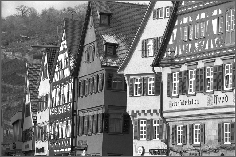
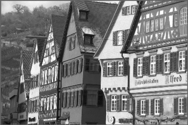
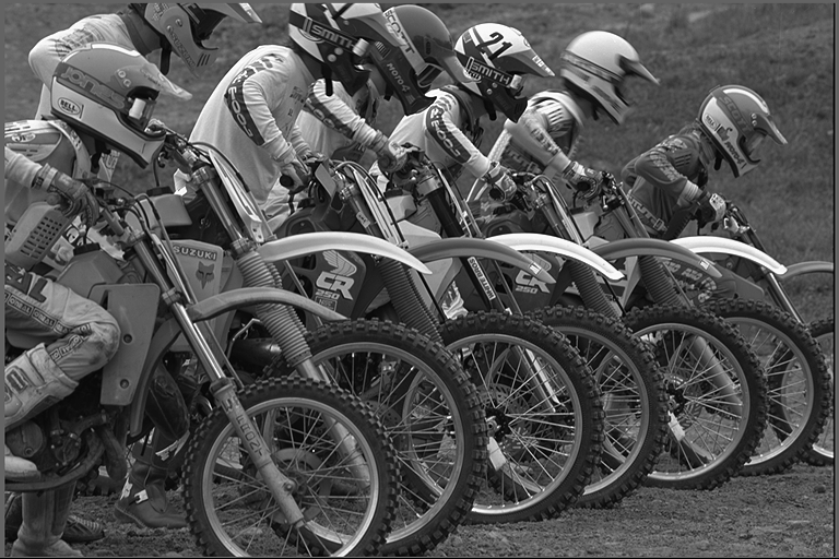
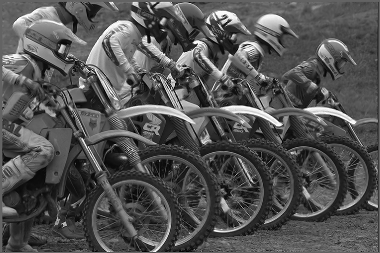
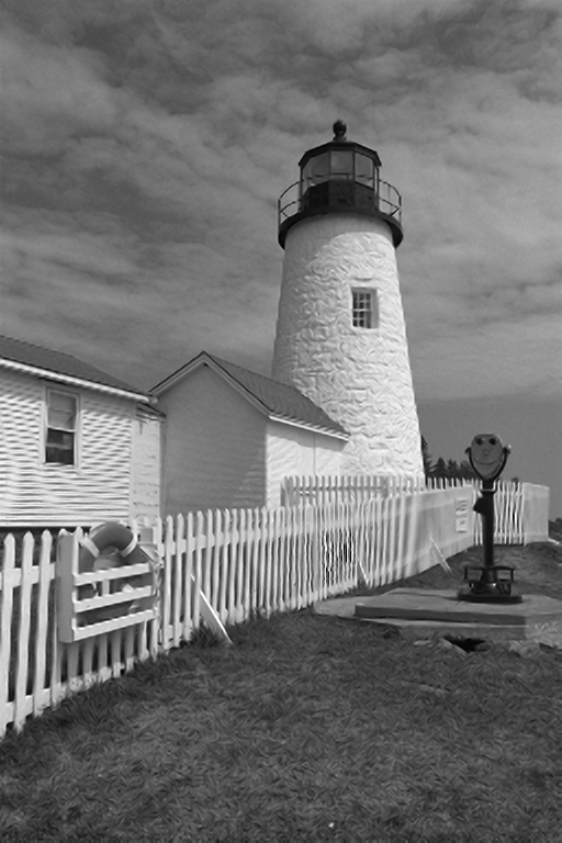
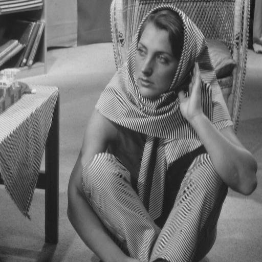
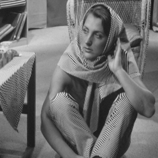
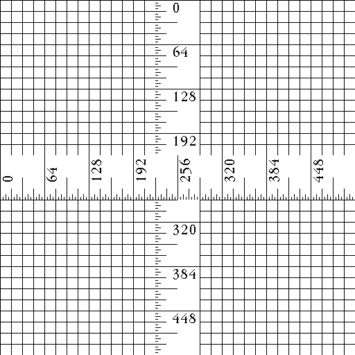
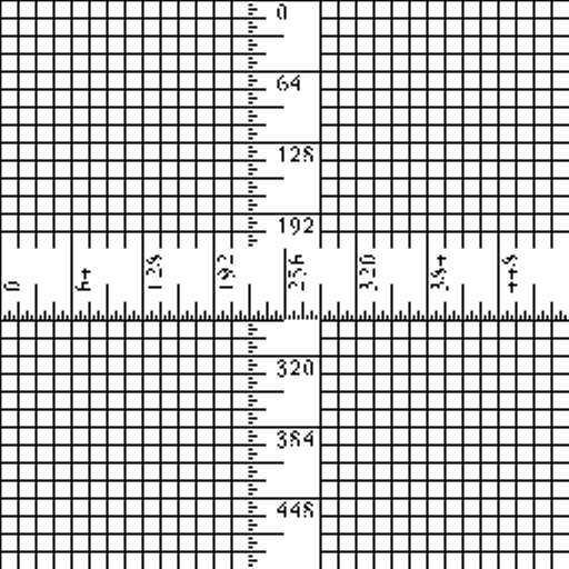
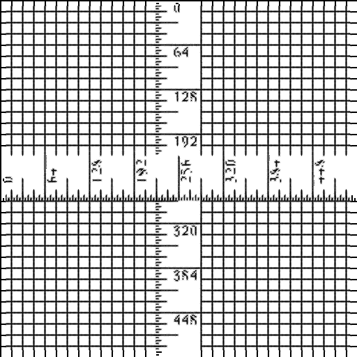
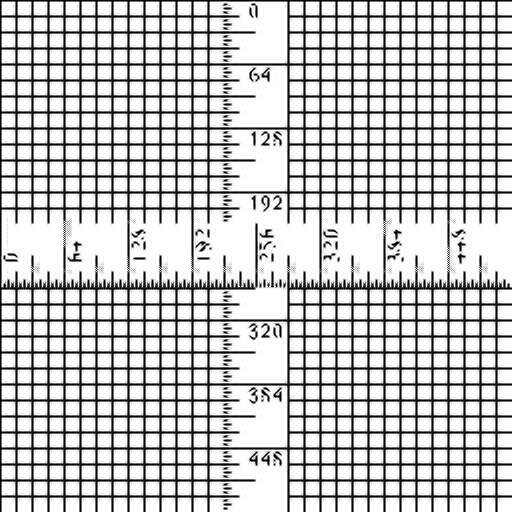
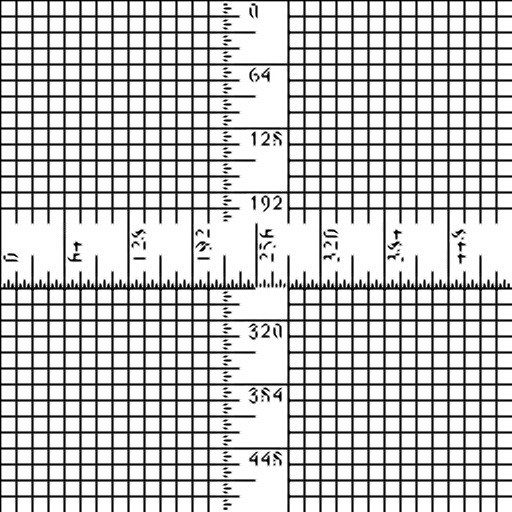
Table 1 tabulates the PSNR results of the four interpolation methods on several images for 2X enlargement. To see the interpolated image of each method, please click the corresponding hyperlink of the PSNR number. The PSNR gains of the proposed method over the best method of other three methods(Bicubic, NEDI, and SAI) are also given in the parenthesis.
Notes: The PSNR results shown in this webpage are computed over the whole image while the results in our ICIP2011 paper are computed discarding the boundary region with 10 pixels width.
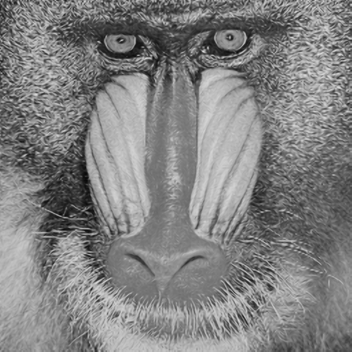
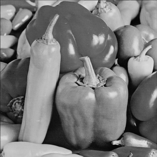
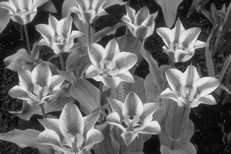
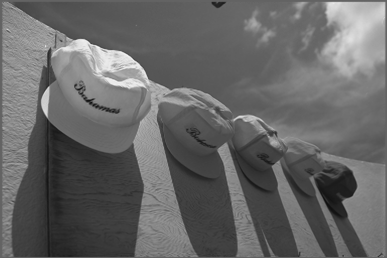
Table 1. PSNR(dB) results of four interpolation methods.
| Images | Bicubic | NEDI[1] | SAI[2] | Proposed | Show Comparison |
|---|---|---|---|---|---|
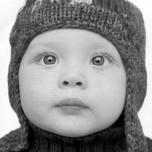
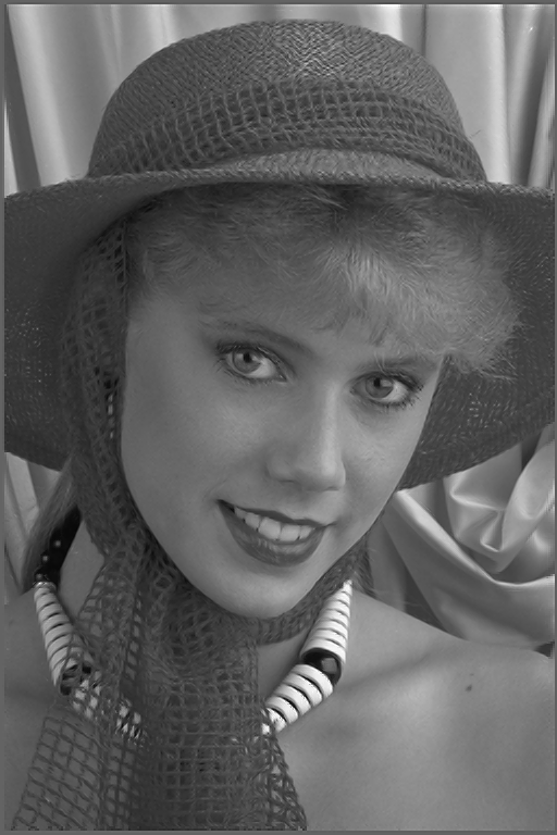
| child | 35.49 | 34.56 | 35.63 | 35.70 (0.06) | Click |
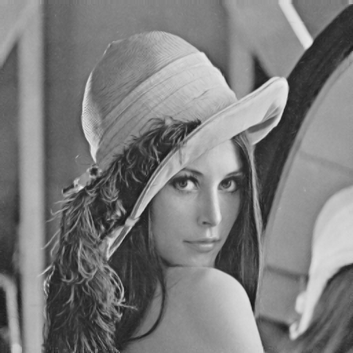
| Lena | 34.01 | 33.72 | 34.76 | 34.79 (0.03) | Click |
| Baboon | 22.47 | 22.55 | 22.70 | 22.69 (-0.01) | Click |
| Pepper | 32.06 | 29.32 | 31.84 | 32.69 (0.63) | Click |
| Tulip | 33.82 | 33.76 | 35.71 | 35.85 (0.14) | Click |
| Cameraman | 25.51 | 25.44 | 25.99 | 26.06 (0.07) | Click |
| Monarch | 31.93 | 31.80 | 33.08 | 33.34 (0.26) | Click |
| Airplane | 29.40 | 28.00 | 29.62 | 30.05 (0.44) | Click |
| Caps | 31.25 | 31.19 | 31.64 | 31.67 (0.02) | Click |
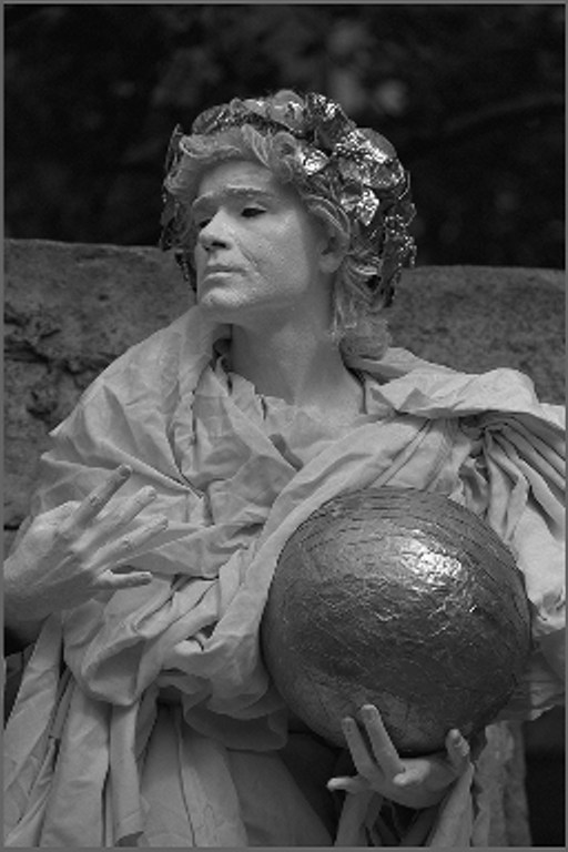
| Statue | 31.36 | 31.01 | 31.78 | 31.94(0.15) | Click |
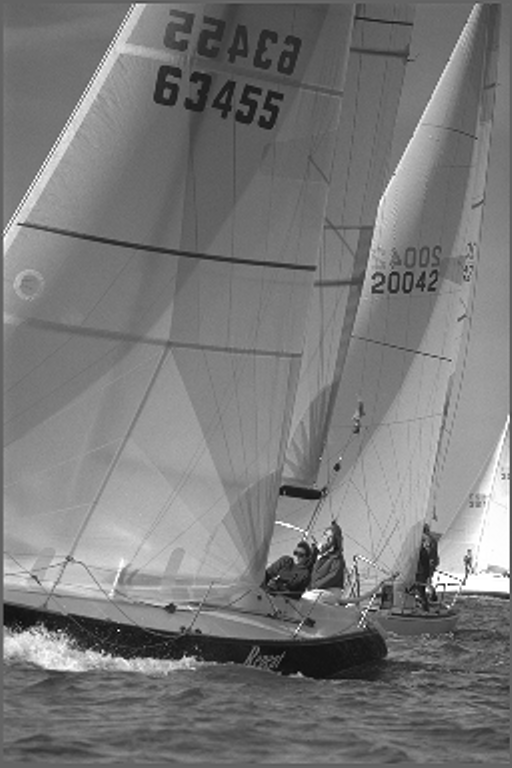
| Sailboat | 30.12 | 30.18 | 30.69 | 30.85 (0.15) | Click |
| House | 22.20 | 21.74 | 22.28 | 22.33 (0.05) | Click |
| Woman | 31.17 | 30.73 | 31.27 | 31.34 (0.08) | Click |
| Bike | 25.41 | 25.25 | 26.28 | 26.31 (0.03) | Click |
| lighthouse | 26.97 | 26.37 | 26.70 | 26.76 (-0.21) | Click |
| barbara | 24.46 | 22.36 | 23.55 | 23.10 (-1.36) | Click |
| Ruler | 11.98 | 11.49 | 11.37 | 11.81 (-0.17) | Click |
| Slope | 26.74 | 26.54 | 26.63 | 26.78 (0.04) | Click |
| Average | 28.13 | 27.56 | 28.42 | 28.56 (0.14) | --- |
Download the test images including the original test images, downsampled LR images, and interpolated images by different methods: alldata.rar ![]()
Notes:
(1) The Bicubic method is labeled as “BC”;
(2) The interpolation method in [1] is labeled as “NEDI”;
(3) The interpolation method in [2] is labeled as “SAI”;
(4) The proposed method is labeled as “IPAR”;
(4) The downsampled LR image is labeled as “LR”;
For example, the interpolation result of the method IPAR on image Lena is labeled as “Lena-IPAR”. Other result images are labeled similarly.
References
[1] X. Li and M.T. Orchard, “New edge-directed interpolation,” IEEE Trans. Image Processing, vol. 10, no. 10, pp. 1521–1527, October 2001.
[2] X. Zhang and X. Wu, “Image interpolation by adaptive 2-d autoregressive modeling and soft-decision estimation,” IEEE Trans. Image Processing, vol. 17, no. 6, pp. 887–896, June 2008.