General Scale Interpolation Based on Fine-Grained Isophote
Model With Consistency Constraint

• Wenhan Yang        yangwenhan@pku.edu.cn
• Jiaying Liu              liujiaying@pku.edu.cn
• Mading Li               martinli0822@pku.edu.cn
• Zongming Guo       guozongming@pku.edu.cn

Published on ICIP, October 2014.

Overview

Interpolation is a general and economic technique for the image enlargement. It generates high resolution image by utilizing low resolution image information with some prior knowledge. Conventional interpolation methods, such as Bilinear and Bicubic, interpolate an image by convolving pixels with a fixed kernel. These methods do not adapt to local structure of images therefore artifacts, such as blurring and ringing, occur in the frontier of different regions.

In order to overcome the above deficiency, edge-directed interpolation methods are proposed. These methods, such as new edge-directed interpolation (NEDI) [1] and soft-decision adaptive interpolation (SAI) [2], pay attention to edge modelling and adapt to local structure. NEDI uses the low-resolution (LR) image covariances to estimate the high resolution (HR) image covariances by a least square problem. Then NEDI estimates HR pixels by their neighbor LR pixels using corresponding covariances. SAI extents the framework of NEDI with a cross-direction autoregressive (AR) model and achieves better performance upon NEDI. These methods have a limitation that they can only deal with the enlargement whose scaling factor is 2ⁱ, (i = 1, 2,...). But the general scale enlargement is required in many scenarios in reality. Thus interpolation methods supporting the general scale enlargement are proposed. Wu et al. [3] proposed an adaptive resolution up-conversion method implemented in H.264/SVC. Two directional AR models constructed of pixels neighbors are used. Li et al. [4] constructed AR models with pixel neighbors instead of their available LR neighbors. The similarity between pixels within a local window is employed to depict the piecewise-stationarity of image signals.

The methods mentioned above embody the neighborhood and edge information in energy function or statistics. Another type of methods identify the edge or isophote direction and interpolate along the direction, such as Wang’s method [5] and segment adaptive gradient angle interpolation (SAGA) [6].

Isophote-Oriented Interpolation

Conventional interpolations generate HR pixels along the image lattice, resulting in unnatural representation of edges. In order to depict the non-stationarity between two regions and keep interpolated edges natural, we introduce isophote. Isophote is a constant intensity line. Stationarity are maintained along the isophote and deviated in its vertical direction. Isophote-oriented interpolation calculates isophotes of images and interpolates along isophotes rather than image lattice to predict HR pixels based on similar stationary regions.

Before generating HR pixel values, an isophote coordinate is established at first. According to the definition of the isophote, we represent an isophote across two adjacent row i and (i + 1) as:

(1)

where I(i,j) is the intensity of LR image pixel located in coordinate (i,j) and α is called displacement coefficient indicating the location where the isophote passing through location (i,j) intersects with row (i + 1) as shown in Fig.2. When the isophote is approximated to a straight line, we can deduce Eqn.(1) with the first-order Taylor expansion:

(2)

Given Eqn.(1), Eqn.(2) reduces to:

(3)

where I_x(i,j) and I_y(i,j) are the first-order derivatives of the intensity at location (i,j). α is deduced from Eqn.(4):

(4)

and the straight line between (i,j) and (i + 1,j + α) determines the isophote cross (i,j). With row i and (i + 1), all these isophotes between LR pixels in row i like (i,j) and connected locations in row (i + 1) like (i + 1,j + α) make up the isophote lattice between row i and (i + 1).

Interpolation can be performed in the isophote lattice when the isophote exactly goes through the HR pixel to be interpolated and two nearby LR pixels as shown in Fig.1. However, in most cases the isophote does not intersect with the image lattice. For interpolation, Data in the image lattice must be projected to the isophote lattice and mapped back to the image lattice when the interpolation along the isophote is completed. In  [5], a directional bilinear interpolation is employed in a parallelogram window consisting of a line parallel with local isophote. In SAGA [6], one dimensional interpolation is applied to grid LR data to the isophote lattice at first and then linear interpolation is employed along the isophote to calculate data value at the “match” location in HR row. Finally one dimensional method is applied again to gridded the data back to the high resolution lattice.

However, two issues are not considered in previous method. First, piecewise-stationary lines cause inconsistent α, which causes undesirable results, such as the image shown in Fig.6. Second, α is determined by I_x and I_y which are easy to be effected by noises, leading to the isophote estimated deviating from the reality.

Fig. 6: Piecewise-stationary lines cause inconsistent α, causing undesirable results.

Interpolation based on fine-grained isophote model with consistency constraint

In order to make the isophote estimation more robust to noises and interpolate in the condition of piecewise-stationary lines, we propose an interpolation algorithm based on fine-grained isophote model with consistency constraint. The proposed algorithm applies a two-layer displacement calculation to make the displacement estimation accurate in fine-grained and a gradient interpolation with consistency constraint to make the displacement estimation consistent in both global-stationary condition or piecewise-stationary condition.

Fig. 2: Flow diagram of the proposed method based on fine-grained isophote model with consistency constraint.

Fig.2 shows the entire work flow of the proposed method including five parts:

• Preprocessing: In order to make use of the isophote information in directions, the input LR images are converted to LR candidates by simple conversions, such as upside down, transpose. The corresponding reverse convertions are performed to HR image candidates before fusion.
• 1-D interpolation: HR pixels located in the line consisting of LR pixels is generated by one dimension interpolation.
• Two-layer displacement calculation: The gradient-based displacement is applied and the local window search displacement is put forward to introduce the fine-grained pixel intensity information to correct gradient-based displacement.
• Gradient interpolation with consistency constraint: A segment gradient interpolation is employed when an interpolated line is stationary while a consistent gradient interpolation is applied to overcome the inconsistent displacement when an interpolated line is piecewise-stationary.
• Adaptive weighting fusion: Adaptive weighting fusion generates HR patches in a fixed non-overlapped window. We utilize the weighting function in the form of formula in  [7] to lower the weight of patches which contains artifacts or noises.

To further explain, we will employ the two-layer displacement calculation, gradient interpolation with consistency constraint and adaptive weighting fusion elaborated in the following subsections.

3.1.Two-Layer Displacement Calculation

The gradient-based displacement is affected by noises or large deviations in the previous row R_i-1 and deviates from real isophotes. The local window search displacement is proposed to compensate and correct the detail of the isophote according to fine-grained pixel intensity information. The local window search displacement is independent with any operator and only related with the specified LR pixel L(i,j) and the (i + 1)-th row R_i+1. Therefore the impact caused by the (i - 1)-th row R_i-1 can be alleviated and the fine detail of the isophote can be preserved. Therefore a two-layer displacement calculation is proposed, including the gradient-based displacement (α₁) calculated as in  [6] and the local window search displacement (α₂).

The approach of calculating α₂(i,j) is to find a location in R_i+1 where the pixel value is or estimated to be the same as the specified pixel L(i,j). Two cases are considered to fulfil the goal.

• Case 1 : Define k indicating a location in R_i+1. Search two adjacent LR pixels L(i + 1,k) and L(i + 1,k + 1) in R_i+1 from center to both sides such that:
  

  Where k satisfies j -W_s < k < j + W_s - 1 and W_s is the size of the search window. If two pixels are found, α₂ is calculated as:

  
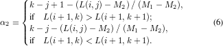
• Case 2 : If there does not exist adjacent pixels in the local search window meeting the required condition, the pixel L(i + 1,k) whose value is most close to L(i,j) is regarded as locating in the same isophote with L(i,j). And α₂ can be calculated as:
  

When α₁ and α₂ are calculated, we simply combine them by a linear summation:

γ balances the weight to control the importance of two items.

3.2.Gradient Interpolation With Consistency Constraint

The displacement α is used to establish the isophote lattice in the gradient interpolation with consistency constraint.

By considering whether an interpolated line is global-stationary or piecewise-stationary, the gradient interpolation with consistency constraint chooses an appropriate interpolation method adaptively. The segment gradient interpolation in  [6] is adopted when the line is global-stationary and the consistent gradient interpolation is applied when the line is piecewise-stationary . The consistent gradient interpolation mitigates the problem without sacrificing the fine detail of the isophote by keeping the displacements of all pixels consistent in a local window for each interpolated pixel.

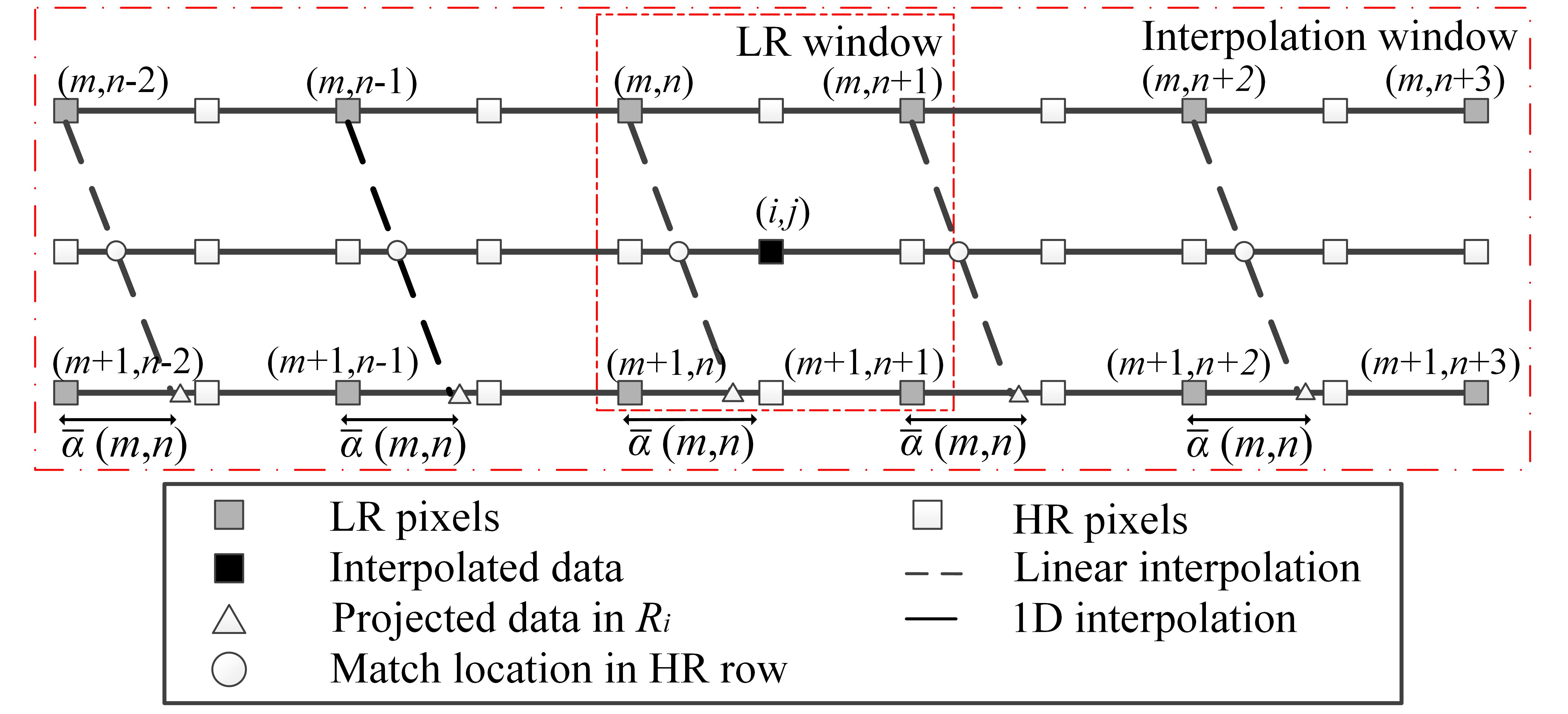
The interpolation is performed in windows and one HR value is generated once. When interpolating H(i,j), we firstly determine its corresponding LR window (consisting of L(m,n),L(m + 1,n),L(m,n + 1) and L(m + 1,n + 1)). α(m,n) , the displacement coefficient of L(m,n) (LR pixel in the upper left corner of LR window), is chosen as the displacement value of the corresponding pixel L(m,n) and five nearby LR pixels in the same row (L(m,n- 2),L(m,n- 1),L(m,n + 1),L(m,n + 2),L(m,n + 3)). α in the interpolation window are set to be consistent and all six LR pixels’ isophote connected locations in the next row is decided by the same α(m,n) instead of their own displacement values. Using the same displacement value only related to the interpolated pixel in the LR window guarantees both consistency and fidelity of the evaluated isophote, as shown in Fig.5. Then the grid projection method in [6] is employed.

3.3.Adaptive Weighting Fusion

After the gradient interpolation with consistency constraint, we get HR candidates in the candidate pool. Then two intuitions are considered to guide the fusion of HR candidates. First, the performances of different interpolations (such as one dimensional interpolation or the gradient interpolation) are different and the weights given to pixels from different interpolations should be handled respectively. Second, the region-based fusion provides more information than the pixel-based fusion and fusion performing in region are better than in pixel. Based on these, we design an adaptive weighting fusion method. First, other than preserving LR pixels exactly locating on the HR lattice, we split HR pixels in HR candidates to clusters by considering their performances. For example, we group the pixels from exactly 1-D interpolation or group the pixels from combination of 1-D interpolation and the gradient interpolation. Second, Fusion is deployed in patch. In order to remove the outlier or noises, we employ a weighting function exp(-x² c) in  [7]. Define P _i (i ∈ 1, 2, 3, 4) as the local patch of intermediate results in the same region and P as the average estimate for the high resolution patch:

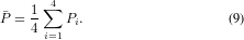
Define w_i as the weight of P_i, the high resolution patch is calculated according to:

where the weighting function w_i is defined as:

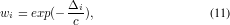
where c is called cliff coefficient, distinguishing whether a value is a noise or outlier. Finally clusters are combined back to a whole image. The procedure is shown in Fig.6.

Experimental results

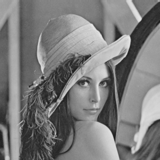
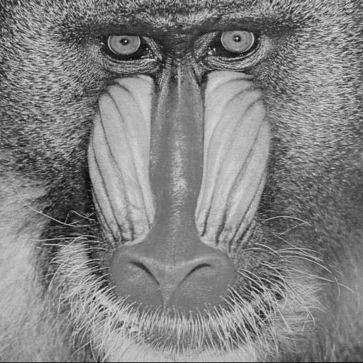
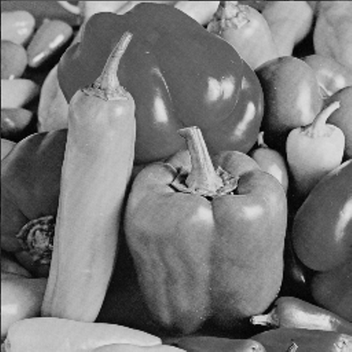
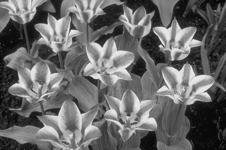
Experiment 1 (Objective Evaluation)

Table 1 tabulates the PSNR results of the interpolation methods on several images for 2X enlargement. To see the interpolated image of each method, please click the corresponding hyperlink of the PSNR number.

Table 1. PSNR(dB) results of interpolation methods.

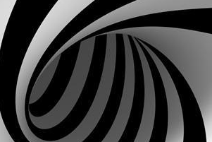
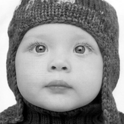
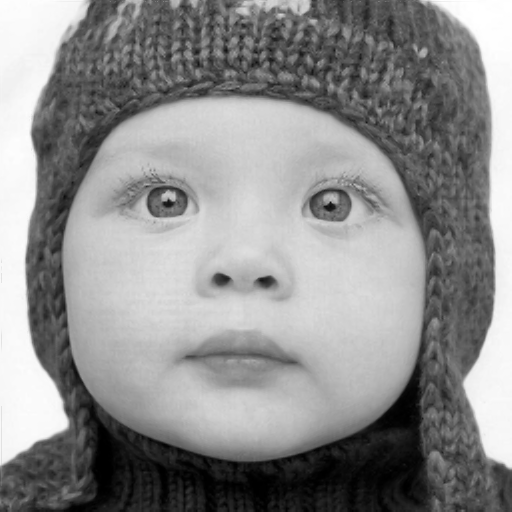
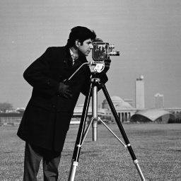
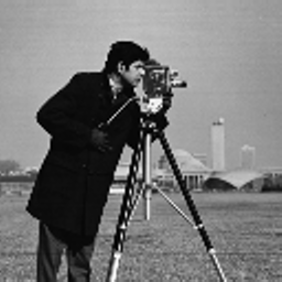
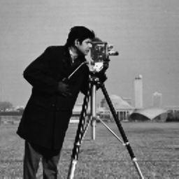
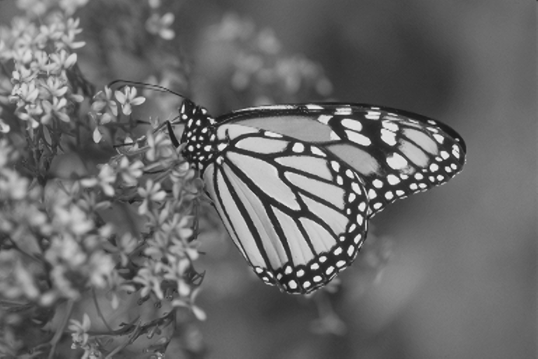
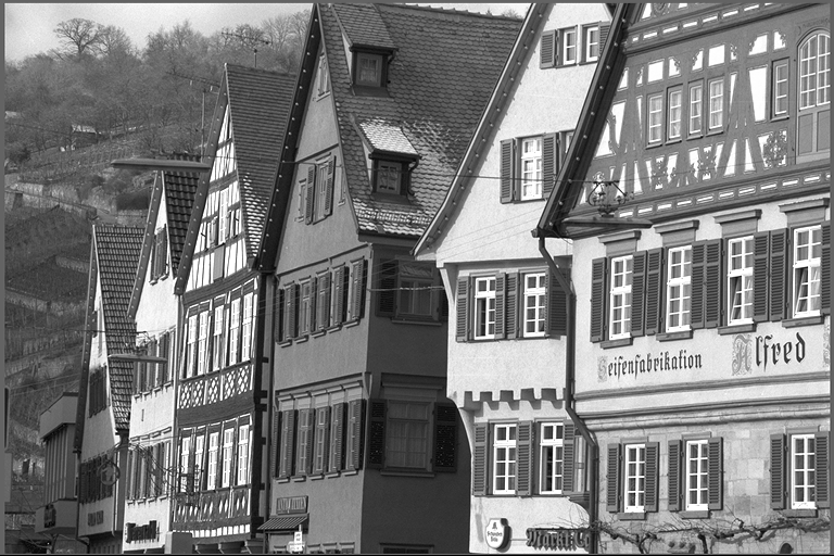
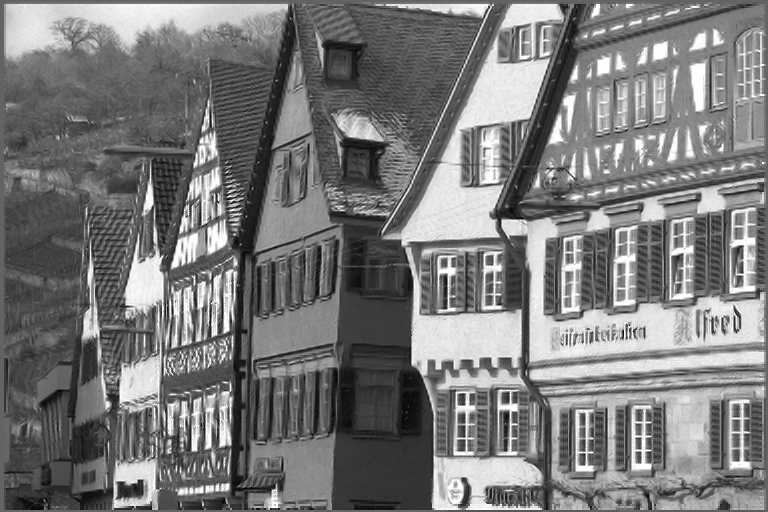
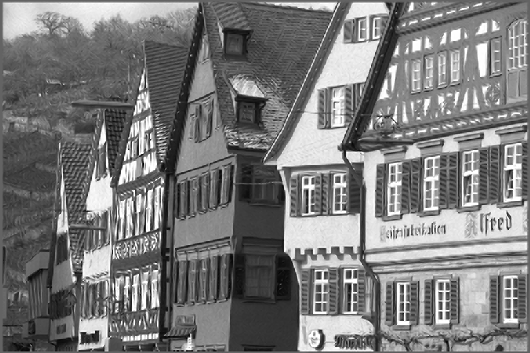
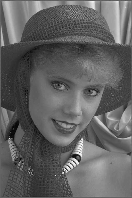
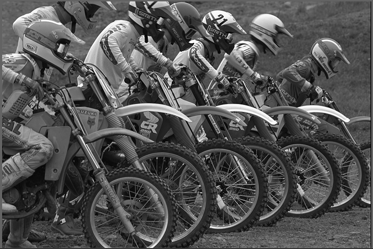
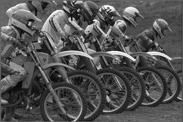
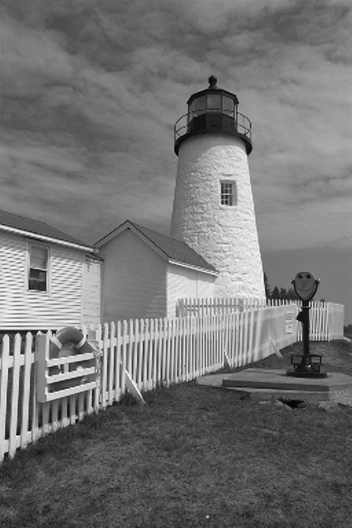
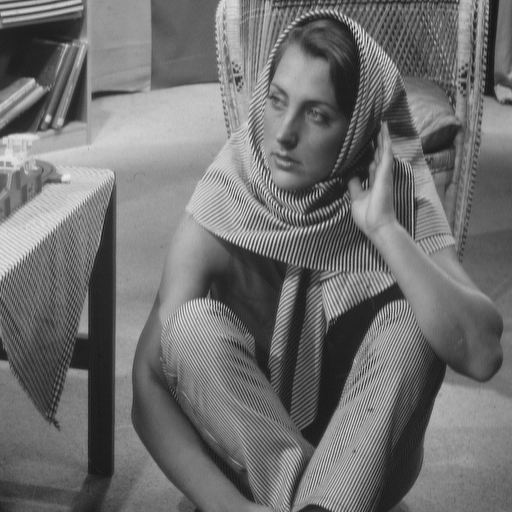
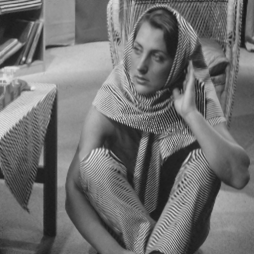
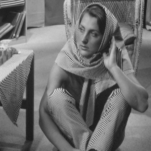
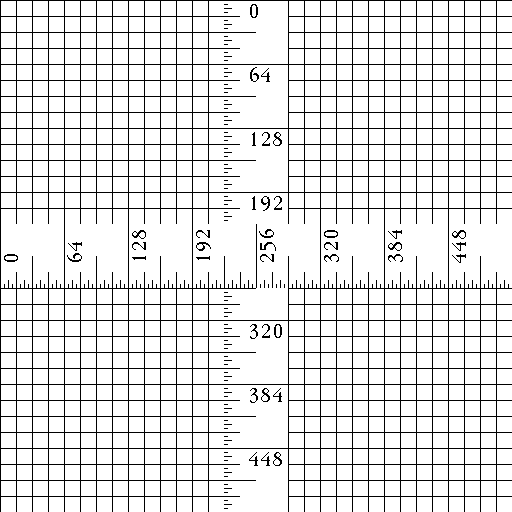
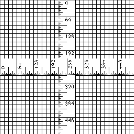
Experiment 2 (Subjective Evaluation)

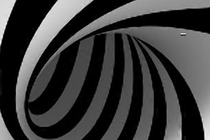Download the test images including the original test images, downsampled LR images, and interpolated images by different methods: ResultImages.zip

Notes

(1) The Bicubic method is labeled as "BC";

(2) The new edge-directed interpolation method in [1] is labeled as "NEDI";

(3) The soft-decision and adaptive interpolation in [2] is labeled as "SAI";

(4) The segment Adaptive Gradient Angle Interpolation in [6] is labeled as "SAGA";

(5) An improved algorithm on SAGA is labeled as "BSAGA". It performs bicubic interpolation where piecewise-stationary lines appear.

(6) The proposed method is labeled as "Proposed";

(7) The original image is labeled as "HR";

References

Back to Projects Page

References

[1] Xin Li and Michael T. Orchard, “New Edge-directed Interpolation,” IEEE Transactions on Image Processing, vol. 10, no. 10, pp. 1521–1527, 2001.
[2] Xiangjun Zhang and Xiaolin Wu, “Image Interpolation by Adaptive 2-D Autoregressive Modeling and Soft-Decision Estimation,” IEEE Transactions on Image Processing, vol. 17, no. 6, pp. 887–896, 2008.
[3] Xiaolin Wu, Mingkai Shao, and Xiangjun Zhang, “Improvement of H.264 SVC by Model-based Adaptive Resolution Upconversion,” in IEEE International Conference on Image Processing (ICIP), 2010.
[4] Mading Li, Jiaying Liu, Jie Ren, and Zongming Guo, “Adaptive General Scale Interpolation Based on Similar Pixels Weighting,” in IEEE International Symposium on Circuits and Systems (ISCAS), 2013, pp. 2143–2146.
[5] Qing Wang and Rabab Kreidieh Ward, “A New Orientation-Adaptive Interpolation Method,” IEEE Transactions on Image Processing, vol. 16, no. 4, pp. 889–900, 2007.
[6] Christine M.Zwart and David H. Frakes, “Segment Adaptive Gradient Angle Interpolation,” IEEE Transactions on Image Processing, vol. 22, no. 8, pp. 2960–2969, 2013.
[7] Pietro Perona and Jitendra Malik, “Scale-Space and Edge Detection Using Anisotropic Diffusion,” IEEE Transactions on Pattern Analysis and Machine Intelligence, vol. 12, no. 7, pp. 629–639, 1990.